In Excel, you can group and ungroup PivotTable dates in order to make data more readable. You can group dates by seconds, minutes, hours, days, months, quarters, and years. I’ll also show you how you can group data by week.
- Click any cell inside a table and insert a PivotTable (Insert >> Tables >> PivotTable).
- Select Date and Units. When you select Date, Excel will automatically add Quarters and Years.
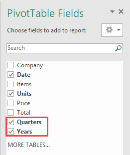
- Uncheck them. Now the data is automatically grouped by months

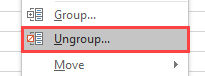
- In order to ungroup it, right-click one of the months and select Ungroup.
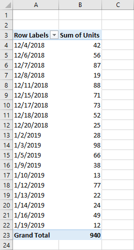
- Now, each day has its own row.
Now, you can group dates the way you want.
Group by years
- Right-click any row inside the date column.
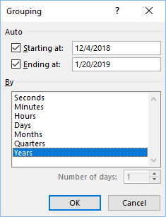
- Click Group.
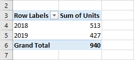
- From the Grouping window, click Years.
The data is grouped into the years 2018 and 2019. Two years are present inside the table.
Group by month
- Right-click any row inside the date column.
- Click Group.
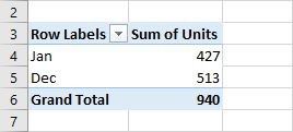
- From the Grouping window, click Months. We have only January and December and these two months will be displayed inside the PivotTable.
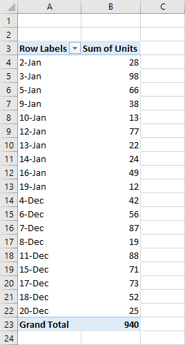
Group by days
Grouping by days displays our data the same way as ungrouped PivotTable because each row in our data represents a single day. Only the way the date is formatted will change.
You can’t change the data formatting easily because the date is not formatted as a date (number really) but as text. If you want to read more about formatting dates in PivotTables, you can read Jon’s article.
Group by weeks
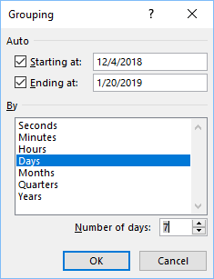
Now, we are going to group dates by weeks, what’s different in this grouping is that you won’t find Weeks in the grouping Window.
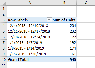
But we know that a week has 7 days, so choose a day and set the number of days to 7.
This is how the result looks like.