In Power Query, you can merge multiple columns into a single one. This is what we are going to do in this lesson.
Import a CSV file and create a table
Navigate to Data >> Get & Transform Data >> From Text/CSV.
Inside the next window, you have two options: Load and Transform Data.
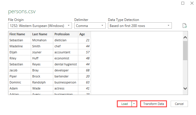
If you click Transform Data, you can modify a table before placing it into a worksheet. But we will insert the data first, and then we are going to merge columns. Click the Load button.
Merge Columns
Now, we have a table inside a worksheet.
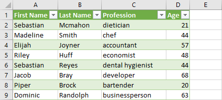
Click the table and navigate to Data >> Get & Transform Data >> From Table/Range.
Now, when we have a Power Query Editor opened you click First Name and (while holding Ctrl) the Last Name.
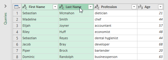
Navigate to Transform >> Text Column >> Merge Columns.
In the next window, you have merge options. You can choose a separator between the merged columns, and a new name for the new column.
Let’s use space as a separator and Name as the name for the column.

If you try to close the Power Query Editor, a new message will pop up.

Press Keep to apply changes.
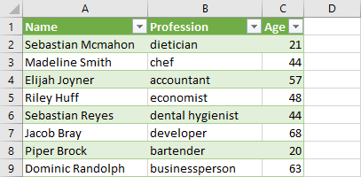
As you can see the table columns merged into one.