Add Data to an Existing Chart in Excel

Sometimes, after we have created a chart in Excel, we may get new data in form of rows or columns of numbers that we need to add to the chart.

The chart we create can either be embedded, meaning that it is on the same worksheet as the source data or the data we used to create the chart, or it can be on a separate chart sheet.

The rows and columns of numbers in Excel that are plotted on a chart are called data series. An example of a data series is the monthly sales of a business.

In this tutorial, we are going to learn how to add new data series to an existing chart: embedded, and also on a separate chart sheet. We will look at how to add new data series to an existing PivotChart.

Add Data Series to an Existing Embedded Chart

Method 1: Use the dragging of sizing handles

We can use dragging to incorporate new data series into an existing embedded chart by using the following steps:

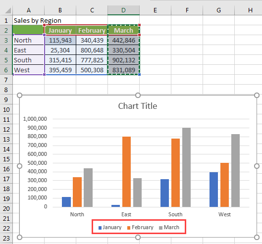
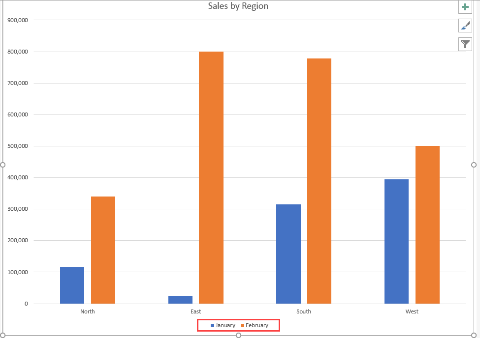
In the example below, the chart displays regional sales for January and February. We have just added a new data series for March. The chart does not yet show the March data series.

1. Enter the new data series in the cells that are directly next to or below the source data for the embedded chart.

2. Click anywhere in the chart. The source data that is currently displayed is selected showing the sizing handles. Please note that the data series for March is not selected.

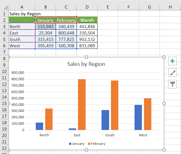
3. Drag the sizing handles in the data source to include the new data. The chart is updated automatically to display the new data series.

Method 2: Update data source by copying and pasting in new data series

We use the following steps to apply this method:

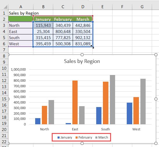
1. Enter the new data series in the cells that are directly next to or below the source data for the embedded chart. In the example below, we have entered the new data series for March.

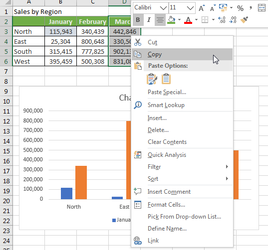
2. Select the new data series and press Ctrl + C to copy. Alternatively, select the new data series and right-click it, and select Copy on the shortcut menu.

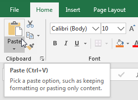
3. Select the chart and right-click it. On the shortcut menu select Paste.

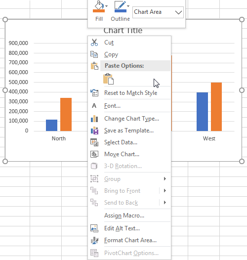
Alternatively, we can click Home >> Clipboard >> Paste.

The chart is updated to reflect the new data series.

Method 3: Update the data source using the Paste Special dialog box

In this method we use the following steps to update the chart data source:

1. Enter the new data series in the cells that are directly next to or below the source data for the embedded chart as we have done before.
2. Select and press Ctrl + C to copy the new data series.
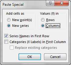
3. Select the chart and click Home >> Clipboard >> Paste >> Paste Special to open the Paste Special dialog box.

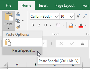
4. In the Paste Special dialog box select Add cells as New series, Values (Y) in Columns, and Series Names in First Row options as follows and click OK.

The chart is updated accordingly to display the new data series.

Add Data Series to an Existing Chart on a Separate Chart Sheet

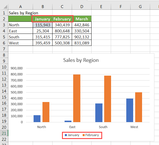
The example below shows the chart on a separate chart sheet that displays the regional sales for January and February.

We can add new data series to the chart by using the following methods:

Method 1: Use the Select Data Source dialog box

Dragging is not the best way of adding new data series to this chart. We can enter the new data using the Select Data Source dialog box.

We use the following steps:

1. Select the worksheet that contains the source data for the chart and in the cells that are directly below or next to the source data, we type in the new data that we want to add.
2. Select the chart sheet that contains our chart.
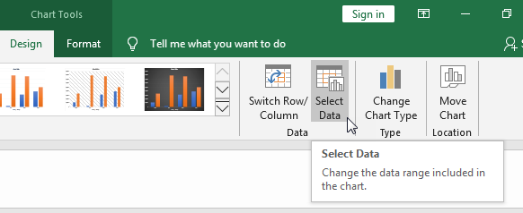
3. To open the Select Data Source dialog box, right-click the chart and click Select Data on the shortcut menu that pops up.

Alternatively, select the chart and click Chart Tools >> Design >> Data >> Select Data.

The Select Data Source dialog box appears in the worksheet that contains the data source.

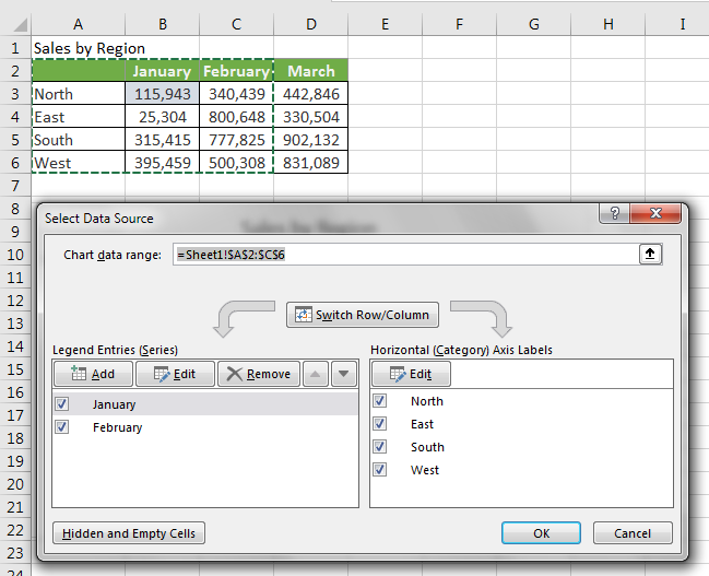
1. With the Select Data Source dialog box still open, click in the worksheet and click and drag to select the entire dataset that we want to use for the chart including the new data that we entered.

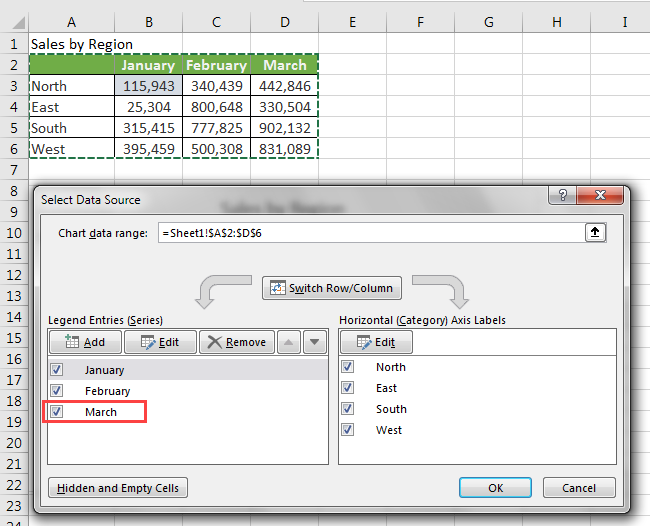
The new data series appears under Legend Entries (Series) area in the Select Data Source dialog box.

5. Click OK to close the dialog box and go back to the chart sheet.

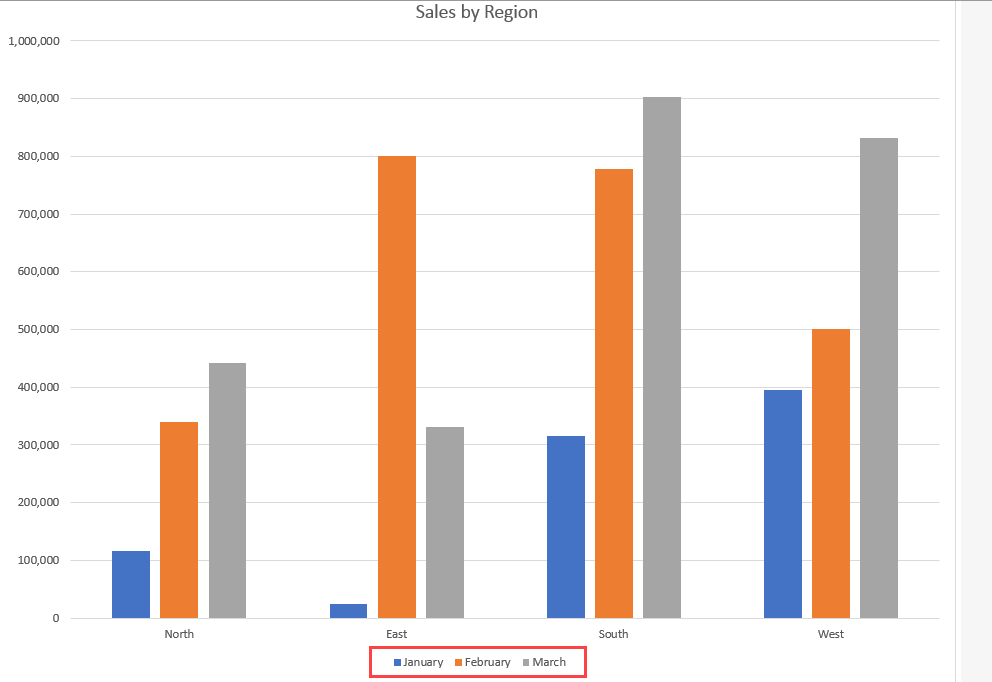
The chart is updated to display the new data series.

Method 2: Update data source by copying and pasting in new data series

In this method, we use the same steps we used in adding data series to an embedded worksheet.

Method 3: Update the data source using the Paste Special dialog box

In this method, we use the same steps we used in adding data series to an embedded worksheet.

Add New Data Series to an Existing Pivotchart

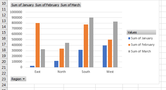
We will use the following PivotChart to show how we can add a new data series to a PivotChart. The chart shows the regional sales for January and February. We want to add the sales for March.

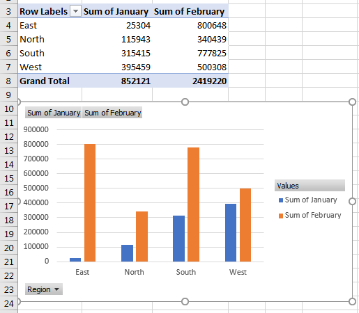
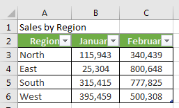
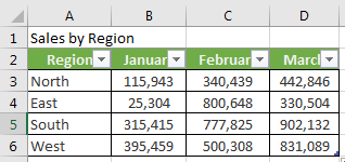
The following is the source data of the pivot table and it is in a different worksheet:

To add the new data series for March we do the following:

1. Select cell D2 and type in the new data as follows:

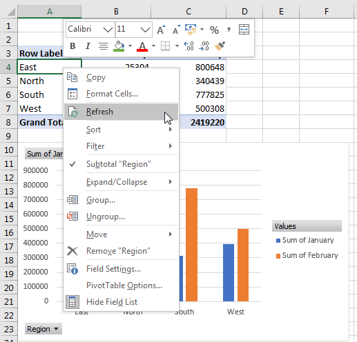
2. Select the worksheet that contains the PivotChart. Right-click any cell in the PivotTable and select Refresh on the shortcut menu.

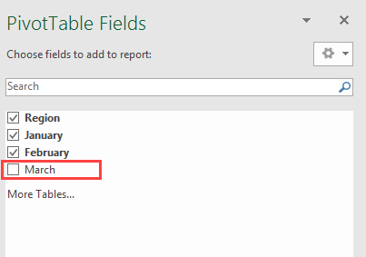
A new field for March is added to PivotTable Fields.

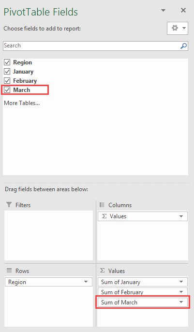
3. Click the checkbox next to March to select it. The Sum of March is added to the Values area of the PivotTables Fields pane.

The PivotChart is then updated accordingly to display the new data series.

Conclusion

In this tutorial we have looked at different methods we can use to add data to an existing chart in Excel.

The chart may be an embedded chart that is contained in the same worksheet as its source data, a chart on a separate chart sheet, or a PivotChart.