Adding horizontal and vertical lines in particular cells of your data set can improve the readability of your data. This tutorial explains how to add horizontal and vertical lines in Excel cells.
We can add horizontal and vertical lines in Excel cells using three methods. We can use the Borders drop-down list, use the Format Cells dialog box, and manually draw the lines.
Example
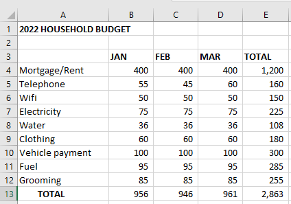
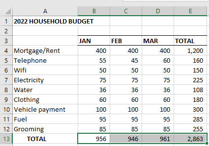
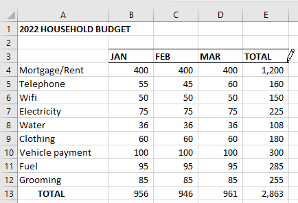
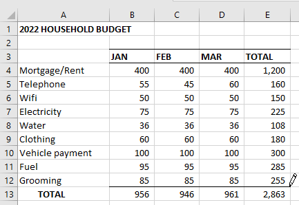
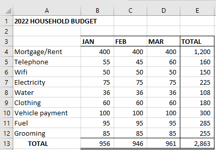
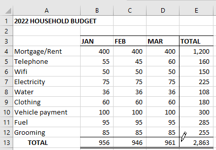
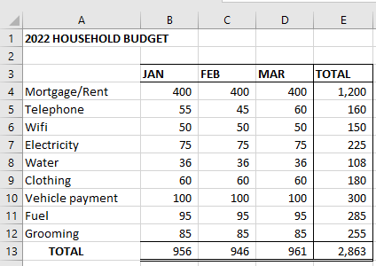
We will use copies of the following data set in our illustrations:
How to add horizontal lines to Excel cells
We will explain the three methods of adding horizontal lines.
Method 1: Use the Borders drop-down list
- Drag the mouse over range B3:E3 to select it.
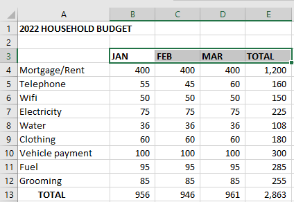
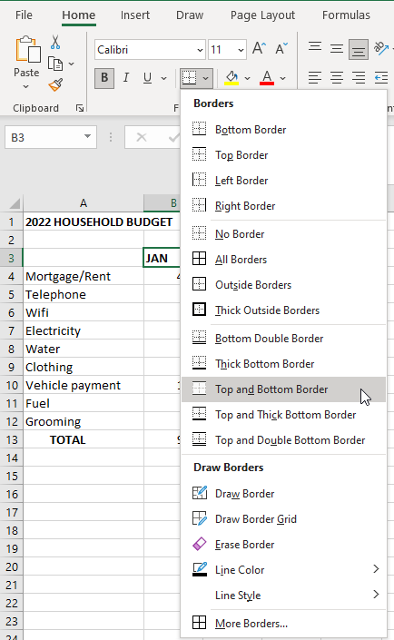
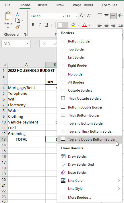
- Click Home >> Font >> Borders Arrow >> Top and Bottom Border.
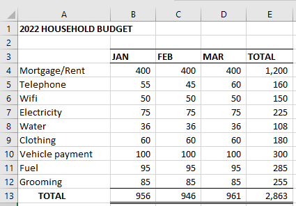
Horizontal lines are added to the top and bottom of the cells in the selected range B3:E3.
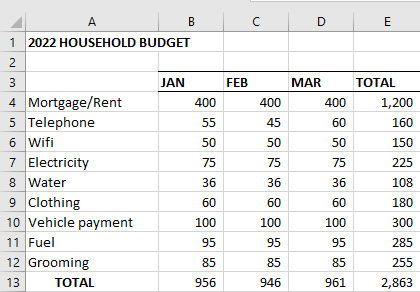
- Drag the mouse over range B13:E13 to select it.
- Click Home >> Font >> Borders Arrow >> Top and Double Bottom Border.
A single line is added to the top of the cells in the selected range B13:E13. A double line is added to the bottom of the cells in the range.
Method 2: Use the Format Cells dialog box
- Drag the mouse over range B3:E3 to select it.
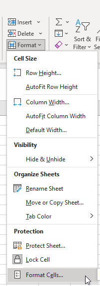
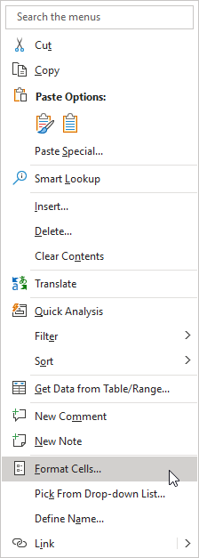
- Click Home >> Cells >> Format >> Format Cells to open the Format Cells dialog box.
Or
Right-click the selected range and click Format Cells on the shortcut menu.
Or
Press Ctrl + 1 on the keyboard.
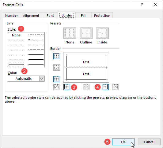
- Do the following five things in the Format Cells dialog box that pops up, in the numbered order:
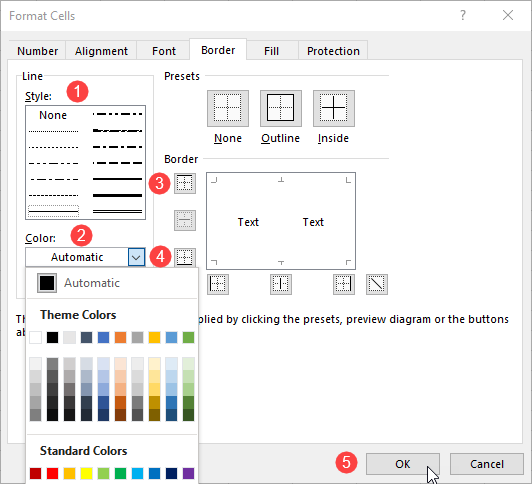
- Choose the style of line you want from the Style box.
- Choose the color you want for the line from the Color drop-down list.
- Click the top border in the Border section.
- Click the bottom border in the Border section.
- Click the OK button to apply the top and bottom horizontal lines.

- Drag the mouse to select range B13:E13.
- Repeat steps 2 and 3 but this time choose a single line style for the top line and a double line style for the bottom line.

Method 3: Draw the lines manually
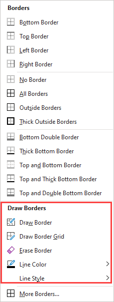
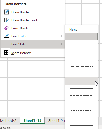
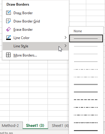
We use the Draw Borders feature of Excel to draw the lines. The Draw Borders options are listed at the bottom of the Borders menu.
We use the followings steps to draw the horizontal lines:
- Choose the line style you want to use.

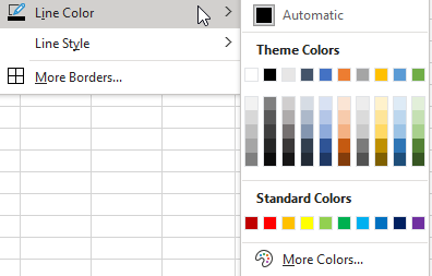
- Choose the line color.

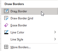
- Click Draw Border.

The mouse pointer changes to a pencil icon.
- Drag and draw single lines along the grid lines on top and bottom of range B3:E3.
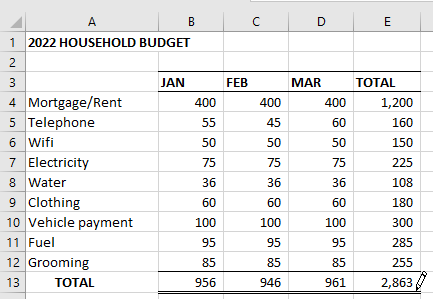
- Drag and draw a single line along the gridline on top of range B13:E13.
- Repeat step 1 but choose a double line style.
- Drag and draw a double line along the gridline at the bottom of range B13:E13.
How to add vertical lines to Excel cells
Method 1: Use the Borders drop-down list
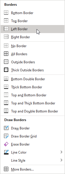
- Select range E3:E13.
- Click Home >> Font >> Borders Arrow >> Left Border.
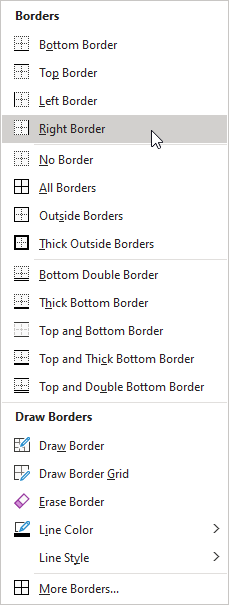
- Click Home >> Font >> Borders Arrow >> Right Border.
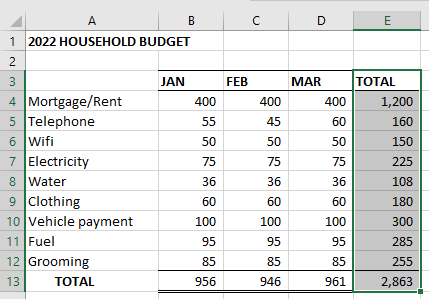
Vertical lines are added to the left and right of the selected range.
Method 2: Use the Format Cells dialog box
- Select range E3:E13.
- Open the Format Cells dialog box as previously explained in this tutorial.
- Select appropriate options in the dialog box. Choose the left and right border in the Border section and click the OK button.
Vertical lines are applied to the right and left of the selected range.

Method 3: Draw the lines manually
- Choose the line style you want to use.
- Choose the line color.
- Click Draw Border.
The mouse pointer changes to a pencil icon.
- Drag and draw a vertical line along the gridline on the left of range E3:E13.
- Drag and draw a vertical line along the gridline on the left of range E3:E13.
Conclusion
Add horizontal and vertical lines to the cells you want to draw attention to in your dataset. This makes your data more readable.
We can add horizontal and vertical lines in Excel cells using three methods. We can use the Borders drop-down list, use the Format Cells dialog box, and manually draw the lines.