Dealing with charts in Excel can be stressful to a lot of people, especially when they are asked to do some things that are out of the ordinary scope.
We will show an example of one of these things- adding a vertical line to Excel charts. We will show how to add the vertical line to a Bar Chart.
Add a Vertical Line to the Bar Chart
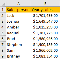
For our example, we will create a table with yearly sales data:
We will present this data on a Bar Chart by selecting the data, then going to Insert tab >> Charts and selecting among Column or Bar Charts:
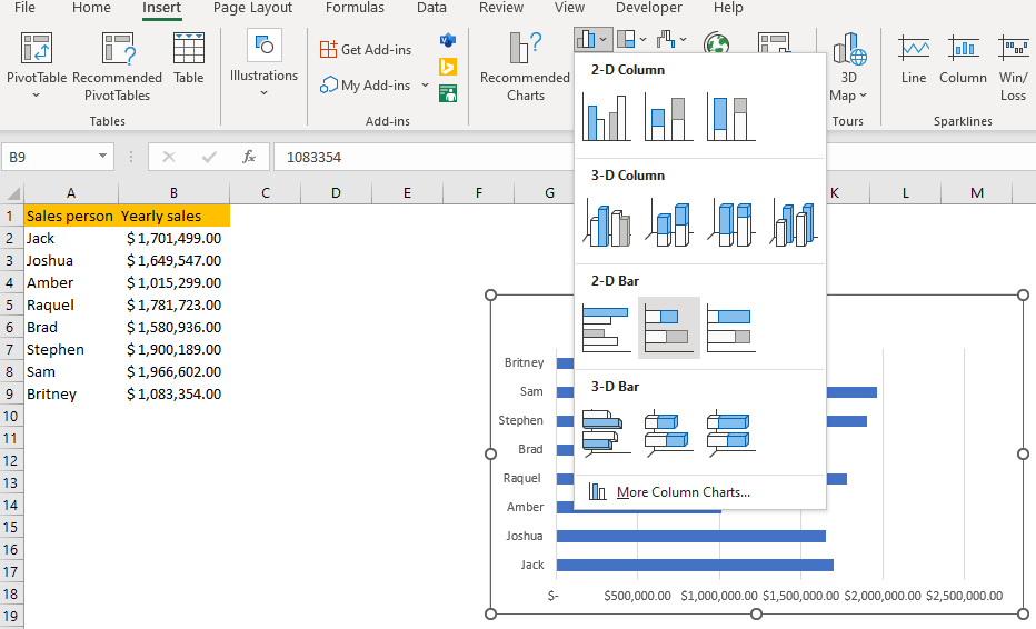
We have purposefully chosen a bar chart as the vertical line would not be as visible in the Column Chart type.
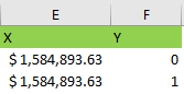
For the vertical line, we will calculate the average sales.
So, once we choose a Bar Chart (2-D Bar Chart in our case), we will create a separate table where we set additional x and y values. X values will be the average of our sales figures, and y values will be set to 0 and 1:
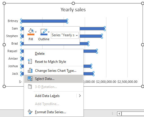
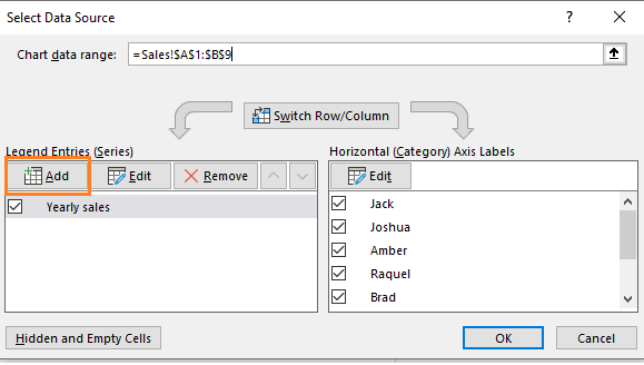
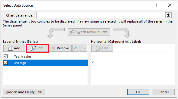
Once we create this mini table, we will go to our chart, right-click on it and choose the Select Data option:
On the pop-up dialog that appears (Select Data Source), we will click the Add button:
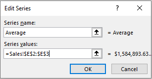
Once on the Edit Series dialog box, we will do the following:
- Select series name in Series name part
- Choose the X values in Series values (range E2:E3 in our case):
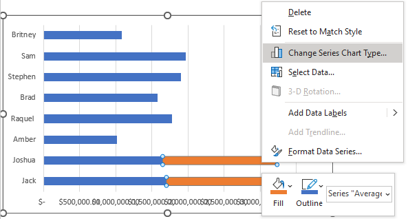
We will click OK two times and will have two bars added to our chart. They will be differently colored. We will select them, right-click on them, and then choose the Change Series Chart Type option:
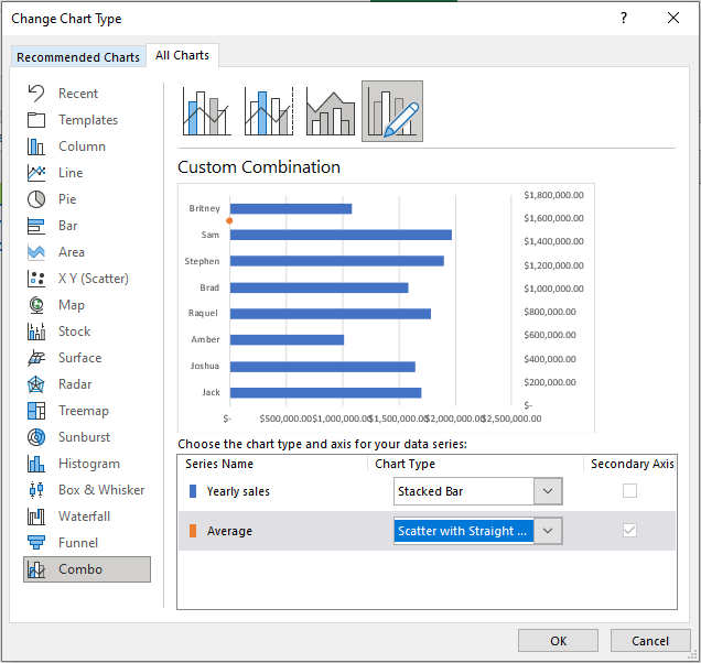
A new window will pop up. In the new window, we will go to the last option- Combo, and choose Scatter with Straight Lines and Markers (one of the XY Scatter charts) for the Average series:
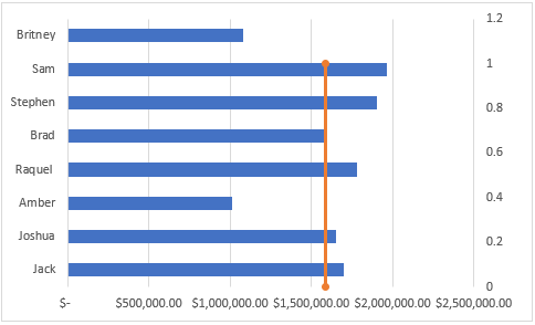
When we click OK, our Average series will be presented as a data point on the y-axis. We will right-click on our chart again, and choose Select Data again.
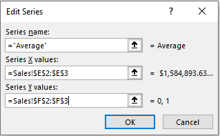
On the Select Data Source window that appears, we will select Average series and click Edit:
In the window that appears, we will leave the name, choose X values (range E2:E3) for Series X values, and choose range F2:F3 for Series Y values:
We will click OK, and we will have a nice vertical line in our chart:
We can now proceed with editing our chart any way we please now.