Apply Conditional Formatting on Multiple Texts in Excel

We already covered a lot of topics about Conditional Formatting in Excel, and along the way proved its usefulness in our daily work.

In the text below, we will show how can we capture multiple texts, i.e. define the rule that will apply to several different values in our range.

Formatting with Common Factor

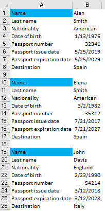
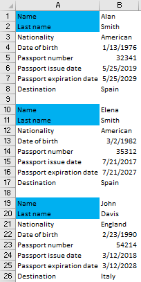
For our example, we will use the table with traveling info for three people, with the data such as passport, destination, passport number, and date of birth.

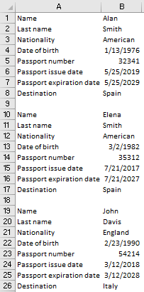
Let us say that we want to highlight the word “Name” in blue color.

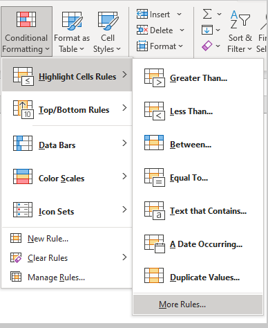
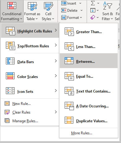
To do so, we will select column A, and then go to the Home tab >> Styles >> Conditional Formatting >> Highlight Cells Rules >> More Rules:

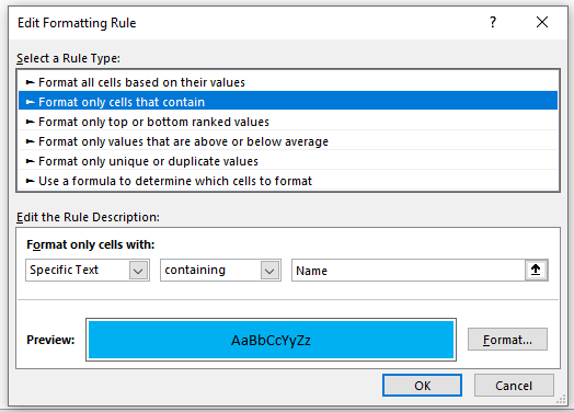
Once we click on it, on a window that appears we need to select Format only cells that contain. Then, in the Edit the Rule Description we have to choose to format only cells with Specific Text (we have this option in a dropdown menu) and then choose beginning with (on a second dropdown menu), and then type in the word “Name” (without quotation marks):

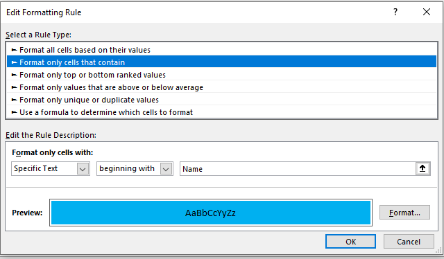
The part “beginning with” is very important, as we also have the word “Last Name” in our range” and we do not want to format these words as well. If we wanted to, we would choose the option “containing”.

Now we have to click on Format, go to the Fill tab, and then choose the light blue option:

When we click OK, we will be returned to the Formatting rule window. We will click OK one more time, and now our table will look like this:

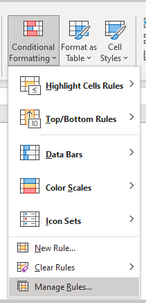
Now let us say that we want to format all the words that contain the word “name”. For this, we will go on and select our first column again, go to Conditional Formatting and then select Manage Rules:

When we click on it, we will see the rule that we defined.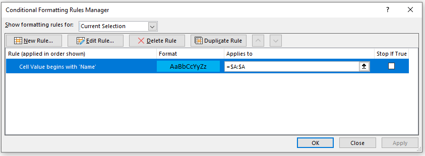

We will click on our rule and then click Edit Rule. We will be prompted to an edit formatting rule window on which we were before. Then we will change the “beginning with” option with “containing” (as we mentioned before):

We have more rows in column A that contain the word “Name” since we have the word “Name” and “Last name” as well. We will input the word „Name“ (notice that this procedure is not case sensitive), and when we click OK, column A will change and these words will be affected:

Formatting with Function

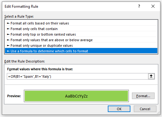
Another way in which we can define the same highlighting rules for different cells i.e. multiple texts is to use functions. Let’s say that we want to highlight the words “Spain” and “Italy” in column B with green color.

We will select column B, go to Conditional Formatting and select New Rule. In the window that appears, we will choose the last option- “Use a formula to determine which cells to format” and input the following formula:

Finally, we will click on Format and select green color under the Fill tab:

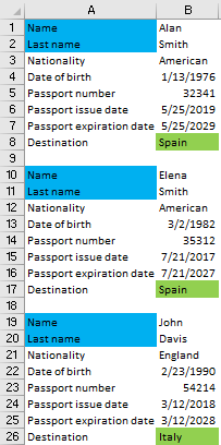
When we click OK, we will see that both desired words are highlighted:

Using Between in Formatting

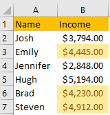
We will create an additional sheet and a table in it with a couple of people’s names and income from $2,500 and $5,500.

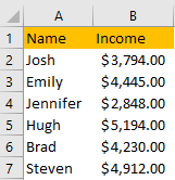
If we want to highlight only those cells in column B between $4,000 and $5,000, we will select the range in this column, and then go to Conditional Formatting >> Highlight Cells Rules >> Between:

Once we click on it, we will define our ranges in a window that appears:

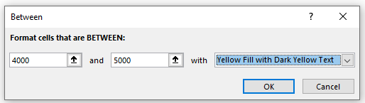
We will define yellow fill for the cells that satisfy our criteria.

Our table will look like this: