Average Only Visible Cells in Excel

When we talk about the calculations in Excel, we have a lot of options at our disposal. We can restrict ourselves in calculations to achieve the desired results.

In the example below, we will show how to use the AVERAGE function to calculate only the cells that are visible, i.e., to omit the hidden cells from the calculation.

Use Average on Visible Cells Only

For the example, we will use the random sales numbers ranging from $100,000 to $300,000, presented in columns A and B:

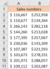
To calculate the average of this range, we will simply use the AVERAGE formula and include the numbers:

And will get the following results:

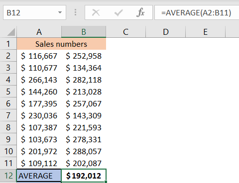
If we would go on and hide any rows at this point (let’s say, rows 3, 8, and 11), the result of our formula would not change, as it reflects the AVERAGE of a particular range, regardless of whether it is visible or not.

There are several ways in which we can find out the average visible range:

1. The first thing that we can do to find the average of our range is to select our visible range, and then the results of several things: sum, average, and the count will be presented in the status bar:

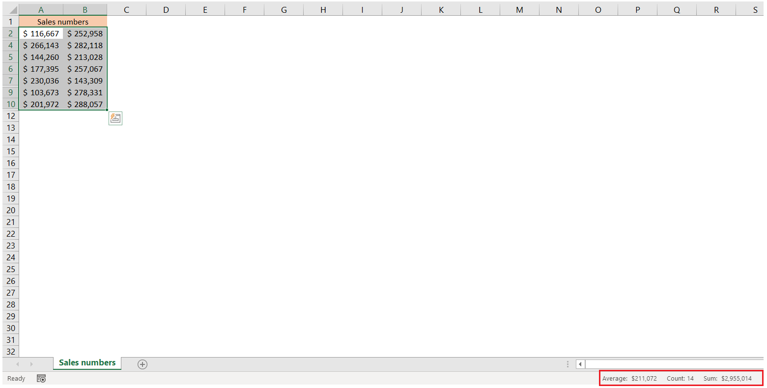
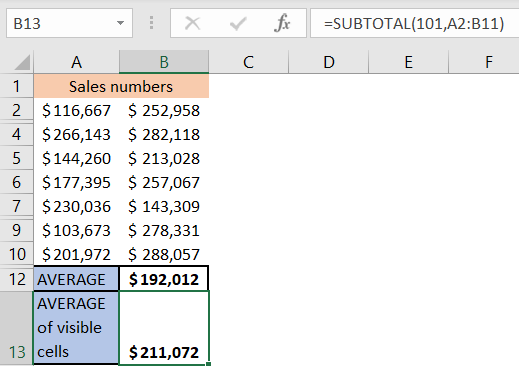
As seen, the average of our visible range is $211,072.

1. Second option is more suitable for our problem and requires less effort in case we are dealing with a larger table. For this purpose, we will use the SUBTOTAL formula, which has two basic arguments:

• Function_num (number of the function that we intend to use)
• Ref1 (our range)

We will insert this formula in cell B12.

For the function number we will choose 101, as this value specifies exactly what we need- calculation of the average of visible cells only.

For our range, we can leave the whole range, but regardless of that, the result will only reflect visible numbers:

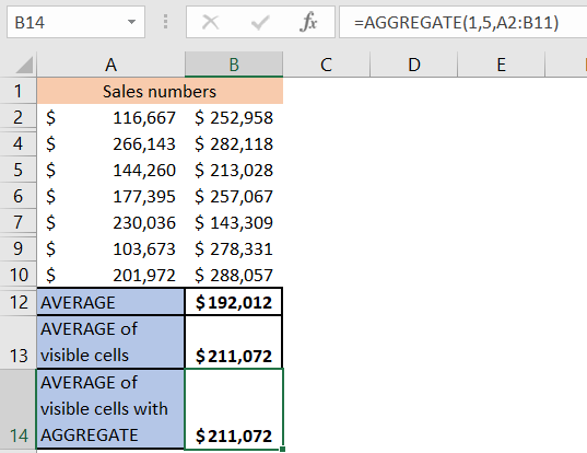
1. Another way to achieve the same result is the use of the AGGREGATE function. This function has three parameters:

• Function_num (a function that we intend to use)
• Options (a lot of ignoring options for a proper calculation)
• Array (our range)

When we start inserting this formula in cell B14, we will first see the list of all available functions:

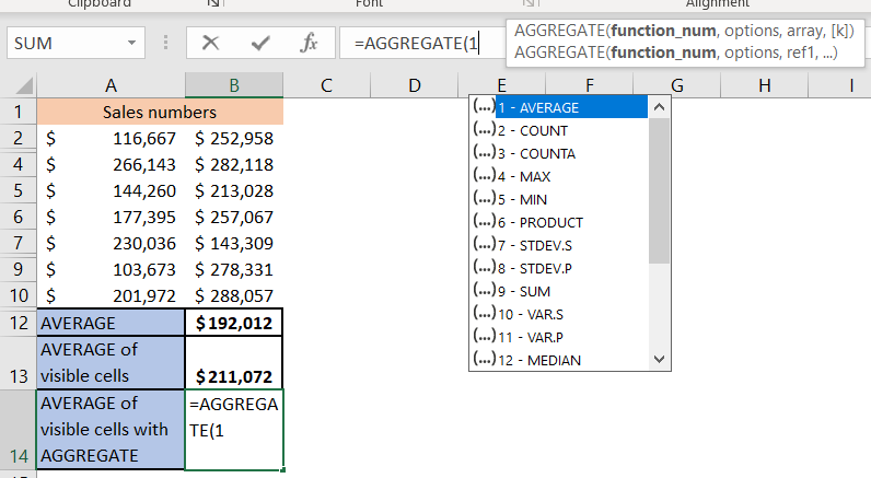
We will choose option 1, for AVERAGE. For the next option, we can choose among a lot of ignoring options:

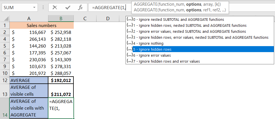
We can find the option that we are looking for at number 5- ignore hidden rows.

For the final step, we will choose the whole range (A2:B11), and will get the result that we are looking for: