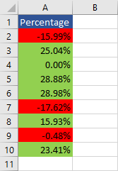
Percent means per cent, and the cent is 1/100 of a dollar. A percent is 1/100 of a whole. Percentages are used in many places: exams, taxes, or discounts.
In this tutorial, we are going to how to use this format in Excel.
Enter a percentage
To calculate the percentage of a number, you just have to insert a number and apply the percentage formatting.
Enter the number 0.5327 into cells A2 and B2.

To convert the B2 value into percentages, you need to apply percentage formatting to this cell. You can find it in the Home >> Number area. Click the Percent Style button.
Remember that 1% = 0.01 = 1/100.

If you hover over the button, you will notice that there is a keyboard shortcut you can use to achieve the same result: Ctrl + Shift + %.

Format cell
There is a number 5 in cell C2, without applied formatting. It has the default general formatting. If you change the formatting to the percentage, Excel will not just add the percentage sign (%), but also converts this number to the percentage value. if 1% is 0.01 and 100% is 1, therefore 500% is 5. This is the result we see after the conversion.

Excel behaves differently if you format a cell before entering a value.
Click cell C2, and enter 5.

When a cell is already formatted, and you want to have 5% inside a cell, you have to enter 5, instead of 0.05.
Remove percentage formatting
To change the formatting from percentage to general, you can select the cells and navigate to Home >> Number.
Now, you can choose the formatting you want. General formatting is at the very top of the list.

Another way to change the formatting to general, is to click any cell that has the default general formatting, and then use the Format painter (Home >> Clipboard >> Format Painter) and select cells with percentages.
Percentage precision
Percentages can be written as integers or decimals. The percentage in Excel is rounded by default, so it doesn’t have a decimal value. You can change it easily by navigating to the Home >> Number area.
There are two buttons you can use to increase or decrease decimal precision: Increase Decimal and Decrease Decimal.

Let’s add two decimal places to the percentage value. Just click the Increase Decimal button twice.

Calculate the percentage of a number
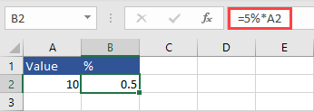
You can multiply a number by a percentage value if you want to know how much is the percentage of the number.
This example shows how much is 5% from 10.
Adding and subtracting percentages
If you want to calculate percentage change by adding or subtracting percentages, it’s tempting to write something like this:

You are going to get 1005.00%. If you convert this number to decimals by choosing the General formatting from Home >> Number, the result is going to look like this:

Excel works differently than a calculator. We didn’t add 5% of 10 to 10, which would result in 10.5. We added 5% of 1 (which is 0.05) to 10 and it gives us the result of 10.05.
If you want to add a percentage of a number to a number, you have to multiply it by the number.

If you want to decrease a number by a percentage, you can use subtraction.

Percentage of a number
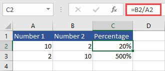
If you want to know what percentage of the first number is a second number, you can use this formula:
|
1 |
= second_number / first_number |
The percentage difference between the two numbers
In the previous step, I showed you how to calculate the percentage of a number. But sometimes we want to know the percentage change between two numbers. It’s used very often in practice, whether you want to calculate rent or tax change, but it’s also useful in many other fields.
Let’s see how it works in practice.
Both formulas return the same result:
|
1 2 3 |
=(B2/A2)-1 =(B2-A2)/A2 |
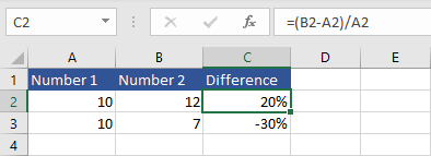
There are two examples, the first example shows the 20% increase, because 12-10 = 2, and 2 is 20% of 10.
The second example shows a decrease of 30%.
Round percentages
You can round percentages to the nearest number, using the ROUND function.

The third example uses parameter 3 as precision for the first digit of a decimal value of a percentage. That’s because this function operates on whole numbers, so 12.3% is 0.123.
That’s easy. But what if you want to round the value to 5 or 0.5 and not to 1 or 0.1.
You can do it similarly as you do with the ROUND function. Even the name of the function is very similar: MROUND.
This function returns a number rounded to the nearest multiple.

If the value is greater than the percentage
Let’s create a formula that will check whether a value is greater than a certain percentage.
This formula displays a text message if the value is greater or equal to 20%.
|
1 |
=IF(A2>0.2, "The value is greater than 20%", "The value is lower or equal to 20%") |

Let’s modify this formula a bit, so we can get a different message if the value is exactly 20%. For this, we are going to modify the formula and create a nested IFs.
|
1 |
=IF(A2>0.2,"The value is greater than 20%",IF(A2=0.2,"The value is equal to 20%","The value is lower than 20%")) |

Percentage ranges
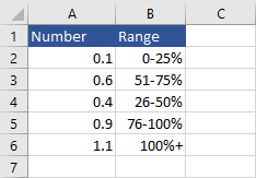
If you don’t want to calculate the exact percentages, but rather check a range that the current number fall into, you can use the following formula:
|
1 |
=IF(A2<=0.25,"0-25%",IF(A2<=0.5,"26-50%",IF(A2<=0.75,"51-75%",IF(A2<=1,"76-100%","100%+")))) |
This formula is more complicated than the one from the last step.
It contains nested IFs and displays 5 ranges from 0 to infinity. You can add more ranges, but the formula will be even more complicated than this one.
Calculate markup percentage
The markup percentage is a difference between cost and selling price.
|
1 |
= (selling_price - cost_price)/cost_price * 100 |
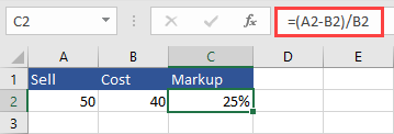
Let’s say that there is a product that you sell for $50, and the cost of this product is $40. You are making $10 by selling the product for $50.
Margin is 10/50 = 20%.
Markup is 10/40 = 25%.
You can easily convert it to an Excel formula.
|
1 |
=(A2-B2)/B2 |
Calculate the average percentage
You can calculate the average percentage the same way you calculate the average number.
|
1 |
= sum(all_numbers)/number_of_value |
The Excel formula is going to look like this:
|
1 |
=SUM(A2:A6)/COUNT(A2:A6) |
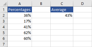
This formula is very simple, but you can use a function that is specifically created to calculate the average value.
|
1 |
=AVERAGE(A2:A6) |
Percentage formula with the TEXT function
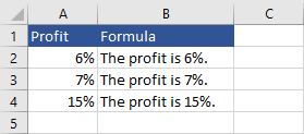
If you try to concatenate the percentage value with text, it will be automatically converted to a number.
Let’s use this function:
|
1 |
="The profit is "&A2&"." |
This is the result you are going to get:
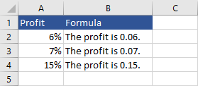
If you want percentages to be displayed as percentages and not as values, use the TEXT function.
|
1 |
="The profit is "&TEXT(A2,"0%")&"." |
The TEXT function takes a value as the first parameter and formats it in the way specified in the second parameter.
Now, if you run this formula it will return the correct result.
Adding zeros for greater precision
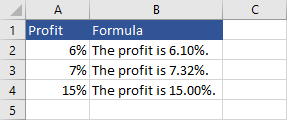
The percentage values in this example (column A) are rounded to the whole number. If you want greater precision, you can modify the formula.
|
1 |
="The profit is "&TEXT(A2,"0.00%")&"." |
Adding two zeros in the decimal place will increase the precision.
Highlighting negative and positive percentages
If you have a big list of percentage values, you may want to differentiate between positive and negative numbers by highlighting negative percentages in red, and 0 and positive in green.
You can do it by using Conditional Formatting.
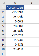
First, select cells with percentage values and go to Home >> Styles >> Conditional Formatting >> New Rule.
Choose Format only cells that contain. In Edit and Rule Description set values as in the picture below.

Click the Format button, and then the Fill tab.
From the Background Color palette choose green and click OK twice.
The first part is done.
Repeat the process by creating another formatting rule this time for values lower than 0. Choose a red color.
