You can modify the individual entries of a chart legend by changing the data inside the worksheet. Besides that, Excel offers options to modify the legend without modifying worksheet data.
You can modify the legend using the Select Data Source dialog box.
I’m going to show you both ways.
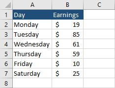
We are going to use a simple example. The following table represents Joe’s earnings.
If you navigate to Insert >> Charts >> Insert Column or Bar Chart >> Clustered Column, you are going to get the following chart.
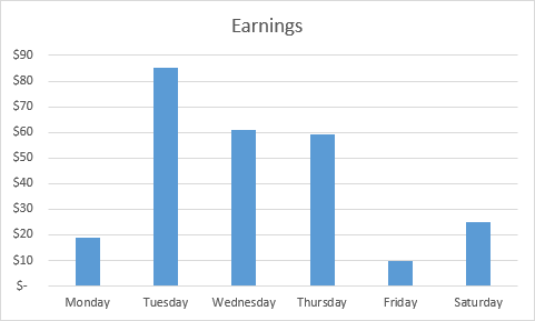
When you try to make the chart narrower, the text under each column won’t fit horizontally, so it will be displayed at an angle.

Edit data on the worksheet
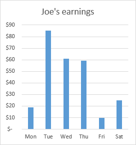
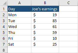
The easiest way to modify the legend is by changing data inside a table. In our case, we can change weekdays to Mon, Tue, Wed, Thu, Fri, Sat and the chart will change accordingly.
You can also change chart title to Joe’s earnings by modifying cell B1.
If you make these changes, the chart will look like this.

Change legend without modifying worksheet data
There is another way to modify chart legend entries, without modifying data inside a table.
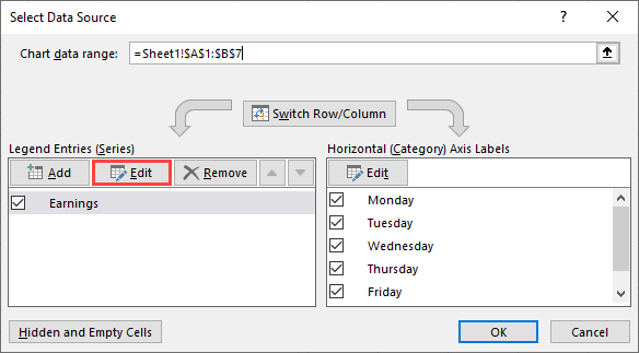
After you create a chart, click it, and navigate to Chart Tools >> Design >> Data >> Select Data.
A new window, called Select Data Source will appear.
Click Edit under Legend Entries (Series).
Inside the Edit Series window, in the Series name, there is a reference to the name of the table.
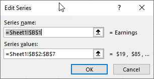
Change this entry to Joe’s earnings and click OK.
Now, click Edit under Horizontal (Category) Axis Labels. Insert a list of names into the Series name box.
={“Mon”,”Tue”,”Wed”,”Thu”,”Fri”,”Sat”}
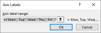
Click OK. Now, the data inside the chart legend is different than the data inside the table.