When you work with Excel, you probably have to deal with data separated into multiple rows. For example name, city, age, etc.
But sometimes you may want to combine cells from two different columns into a single column – for example, you have the First Name and Last Name columns and you want to merge them into a single Name.
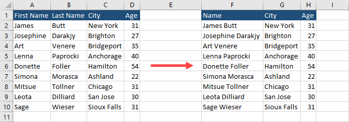
Ampersand (&)
One of the quickest and most popular ways to combine two cells into one is by using an ampersand (&).
We are going to check it on our example and try to concatenate the first and last names into a single column.
Here’s what our example looks like.
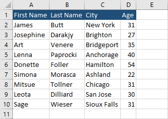
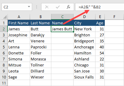
Insert a new column between rows B and C and call it Name. In cell C2, enter the following formula:
|
1 |
=A2&" "&B2 |
It means: join A2 with space and with B2.
Autofill the rest of the cells in the column.
Now, if you try to remove columns A and B, you are going to get the reference error.
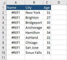
It happens because the cells are not values, but formulas referencing to cells you’ve just canceled. What you have to do before canceling these cells, is to convert them to values.
You can easily do it by clicking cell C2 and using the Ctrl + Shift + Down Arrow keyboard shortcut. It will select all the cells inside that column, without a header.
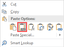
When you have these cells selected, copy them (Ctrl + C), right-click to open the contextual menu and click the Paste As Values button.
The CONCAT function
The CONCAT function is the same as CONCATENATE. CONCAT is the newer version, and you should use it instead of CONCATENATE. This function can merge up to 30 text items together and return the result as text.
Here’s what you need to insert into cell C2 if you don’t want to use ampersand.
|
1 |
=CONCAT(A2," ",B2) |
The result is exactly the same.
Combine text with numbers
You can easily combine text with numbers. There is no need to change the data type Excel will take care of that.
Let’s try this example.

Try this formula:
|
1 |
=A2&" "&B2&" is "&D2&" and lives in "&C2&"." |
This is what it looks like with CONCAT.
|
1 |
=CONCAT(A2," ",B2," is ",D2," and lives in ",C2,".") |
Both methods return this message:
|
1 |
Art Venere is 31 and lives in New York. |
Combine text with dates
It’s a bit more complicated when it comes to dates.
Let’s try it on the following example.
Run this formula.
|
1 |
=A2&" "&B2&" was born in "&D2&" and lives in "&C2&"." |
This is the result it returns.
|
1 |
Art Venere was born in 32363 and lives in New York. |
You can try to run the CONCAT function.
And it will give you the same result.
The problem is that Excel stores dates as numbers and convert them to dates. If you try to concatenate the date it will display a number instead.
You can modify the formula, so it will display a date instead of a number. Here’s how to do it.
|
1 |
=A2&" "&B2&" was born in "&TEXT(D2,"mm/dd/yyyy")&" and lives in "&C2&"." |
|
1 |
=CONCAT(A2," ",B2," was born in ",TEXT(D2,"mm/dd/yyyy")," and lives in ",C2,".") |
This is the result.
|
1 |
Art Venere was born in 08/08/1988 and lives in Bridgeport. |
You can also use just a year, instead of the full date.
|
1 |
=A2&" "&B2&" was born in "&YEAR(D2)&" and lives in "&C2&"." |
|
1 |
=CONCAT(A2," ",B2," was born in ",YEAR(D2)," and lives in ",C2,".") |
Result:
|
1 |
Art Venere was born in 1988 and lives in Bridgeport. |
Use notepad to combine cells
Another way you can easily combine cells is to use a notepad. Copy the first and last names (A2:B10), and paste them into the notepad.

Now, if you copy contents inside a notepad, you are going to have the first name and the last name in different columns.
What you have to do, is to copy a tab between the first and last name. Press Ctrl + H to open the Replace window.
Copy the tab into the Find what textbox, and type space into Replace With.
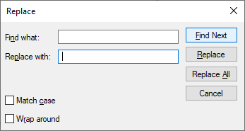
Click the Replace All button.
Now, instead of tabs between words, you have spaces.

Copy everything and paste it into a column.
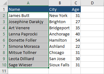
Because there are no tabs between words, Excel doesn’t move them into separate cells.
Separators (space, dash)
Now, let’s talk about separators. Usually, the separators between words are spaces.
|
1 |
=A1&" "&B1&" "&C1&" "&D1&" "&E1&"." |

If you want to use a different separator, for example, a dash, you can replace all spaces with dashes.
|
1 |
=A1&"-"&B1&"-"&C1&"-"&D1&"-"&E1&"." |
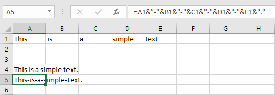
Changing each separator is very tedious, so instead of adding separators between each word, you can insert a space into cell A2 and use the following formula.
|
1 |
=A1&A2&B1&A2&C1&A2&D1&A2&E1&"." |
This will give us the same result as before.
If you want a dash as a separator, you have to add an apostrophe before the dash, otherwise, Excel will treat this as a formula. Apostrophe tells Excel that it should treat everything in that cell as text.
Type this into cell A2.
|
1 |
‘- |
Now, the text changed to:
|
1 |
This-is-a-simple-text. |
Separators (line break)
If you want to separate words into different rows, you have to use line breaks. You can’t add line breaks using a keyboard, at least not directly.
To achieve it you have to get a character from the character set. A line break is number 10.
Let’s create a formula to split the words into new lines.
|
1 |
=A1&CHAR(10)&B1&CHAR(10)&C1&CHAR(10)&D1&CHAR(10)&E1 |
When you execute the formula, you will notice that it didn’t change a thing.
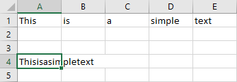
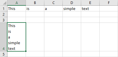
But when you navigate to Home >> Alignment, there is a feature called Wrap Text. Click it, and It will wrap text in the exact places the CHAR(10) functions are inserted.
Creating a VBA function (Separators)
Even if you add a separator to a cell, you have to remember where the separator is, or lock cells, so you won’t delete it by accident. It’s still not the best option.
Where Excel is not enough, VBA will take care of it. That’s why we are going to create a function that will help us to deal with the problem.
First, open the VBA code editor (Left Alt + F11) and create a new module.
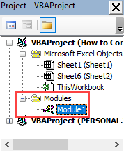
Inside this module insert the following code.
|
1 2 3 4 5 6 7 8 9 10 11 12 13 14 15 16 17 18 |
Function CONCATSEP(ParamArray var() As Variant) As String Dim i As Integer Dim result As String Dim separator As String separator = var(UBound(var)) If UBound(var) > 1 Then For i = LBound(var) To UBound(var) - 1 If i > 0 Then result = result + separator + var(i) Else result = result + var(i) End If Next End If CONCATSEP = result End Function |
Code explanation:
We use ParamArray var() As Variant because we don’t know how many arguments will be inside the function. This allows us to take any number.
separator = var(UBound(var)) – This part of the code get values from the last element and assigns it to the separator variable.
If UBound(var) > 1 Then – If there are at least three arguments (two strings + separator) use the code inside. Counting starts from 0 and then 1, 2. That’s why we are talking about three arguments and not two.
Inside the If function, the program checks whether we are dealing with the first argument. We don’t want to add a separator at the beginning of the first argument, because it will return a string with the separator at the beginning.
