Sometimes you may want to concatenate or join values of a PivotTable. This tutorial shows you three techniques for concatenating the values of a PivotTable.
How to Concatenate Values of a PivotTable
Method 1: Use the Ampersand (&) Operator
In this method, we use the ampersand operator to concatenate values of a PivotTable.
The ampersand operator combines several text strings into one text string.
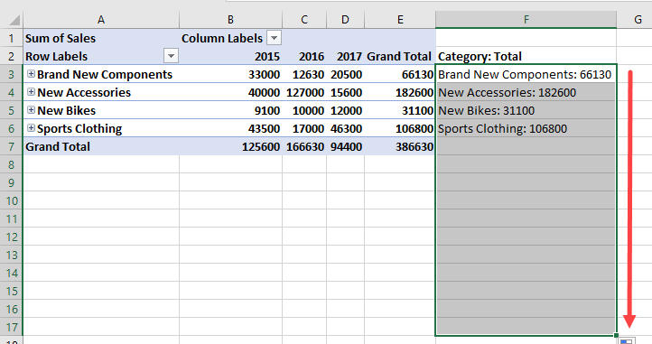
Suppose we have the following PivoTable that summarizes the annual sales of certain product categories.

We want to concatenate the values in Column A and Column E in Column F using a colon (:) delimiter.
We use the following steps:
- Select cell F3 and enter the following formula:
|
1 |
=IF(AND(A3<>"",A3<>"Grand Total"),A3 & ": " & E3,"") |

- Drag down the fill handle to copy this formula down the column way beyond the end of the PivotTable. This ensures we get concatenated values for any new data that may be added to the PivotTable.

Explanation of the formula
|
1 |
=IF(AND(A3<>"",A3<>"Grand Total"),A3 & ": " & E3,"") |
- The IF function uses the AND logical operator to check that cell A3 is not blank and does not contain the “Grand Total” text string.
- If the AND logical operator returns TRUE, the values in cell A3 and cell B3 are combined and returned as one text string in cell F3.
- If the AND logical operator returns FALSE, the IF function returns an empty string in cell F3.
Method 2: Use the CONCAT Function
In this method, we use the CONCAT function which concatenates or joins a range or list of text strings.
Suppose we have the following PivoTable that summarizes the annual sales of certain product categories.

We want to concatenate the values in Column A and Column E in Column F using a colon (:) delimiter.
We use the following steps:
- Select cell F3 and enter the following formula:
|
1 |
=CONCAT(A3,": ",E3) |

- Drag the fill handle down to copy the formula to cell F6. We do not copy the formula to the Grand Total row.

Note: If new rows of data are added to the PivotTable, we would need to copy the formula to those rows excluding the Grand Total row.
Method 3: Use the TEXTJOIN Function
In this method, we use the TEXTJOIN function which concatenates a range or a list of text strings using a delimiter.
Suppose we have the following PivoTable that summarizes the annual sales of certain product categories.

We want to concatenate the values in Column A and Column E in Column F using a colon (:) delimiter.
We use the following steps:
- Select cell F3 and enter the following formula:
|
1 |
=TEXTJOIN(": ",TRUE,A3,E3) |

- Drag the fill handle down to copy the formula to cell F6. We do not copy the formula to the Grand Total row.

Note: If new rows of data are added to the PivotTable, we would need to copy the formula to those rows excluding the Grand Total row.
Conclusion
This tutorial has explained three techniques for concatenating values of PivotTable. We can use the ampersand operator, the CONCAT function, or the TEXTJOIN function.
