Conditional Formatting Based on Date in Excel

Conditional Formatting is one of the best tools that can help us to highlight our cells and help us visually represent our data.

Formatting can be determined by many factors, such as range, value, a specific text, or even a date. In the example below, we will show the latest formatting option we mentioned- formatting by a date.

Conditional Formatting with Date Occurring

For our example, we need data that will have actual dates. We will use the table with sales figures and the dates when they were achieved:

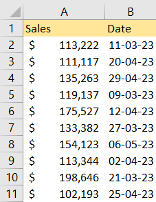
These dates are in the span of two months before the date this article was written (7th of May, 2023). To find out which sales were made in the previous month, we can either use a formula (subtract today’s date by 30) or highlight these cells with Conditional Formatting.

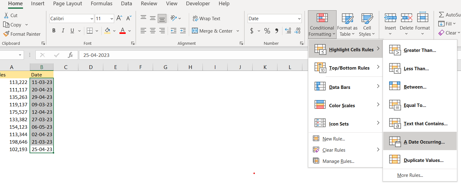
To do the latter, we will go to Home tab >> Styles >> Conditional Formatting >> Highlight Cells Rules >> A Date Occurring:

Once clicked, the window for formatting will appear. In this window, we will choose Last month under Format cells that contain a date occurring, and we will choose the formatting option in a dropdown on the right side (in our case- Light Red Fill with Dark Red Text):

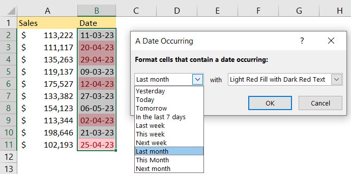
Since we chose Last month, only the dates of sales that refer to the last month will be highlighted.

The problem, or the good thing with this formula, depending on how you look at it, is that it calculates the date based on today’s date, so our highlighted cells can change as today’s date changes.

Conditional Formatting with New Rules

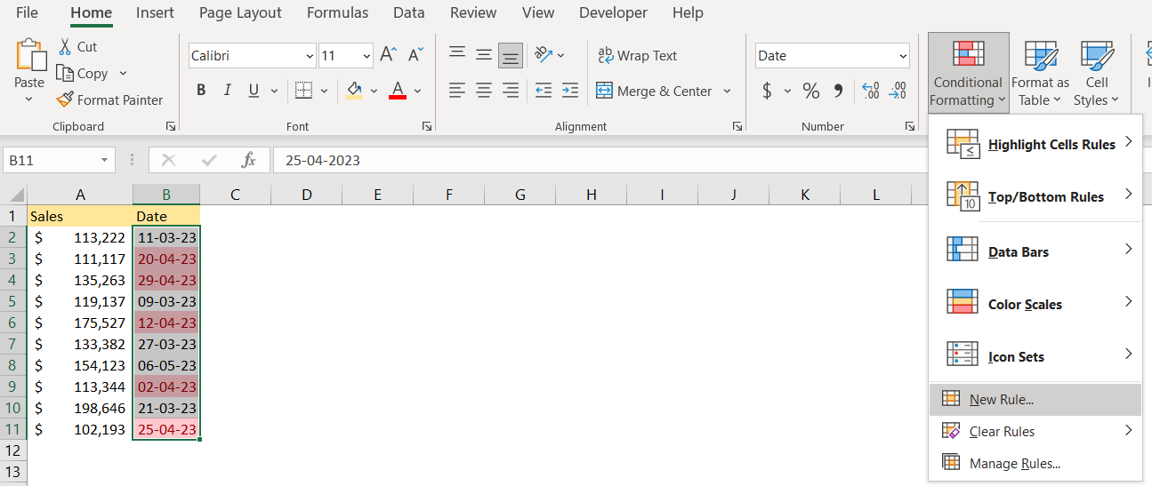
We can use fixed formatting for dates as well. To do this, we will select our range, then go to the Home Tab >> Styles >> Conditional Formatting >> New Rule:

Under the window that appears, in Select a Rule Type we will choose Use a formula to determine which cells to format option. Under that option, in Edit the Rule Description, we will insert the formula:

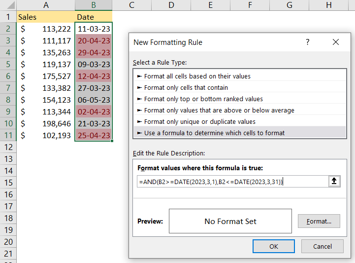
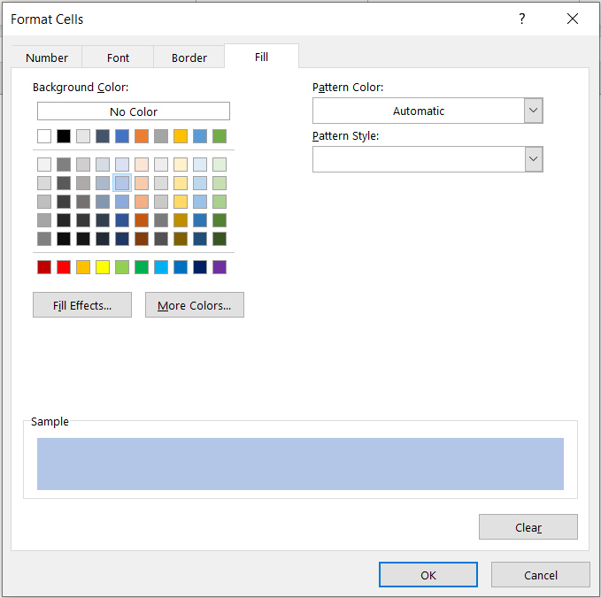
This formula will encompass all the dates in March (higher or equal to March 1st, and lower or equal to 31st of March). We need to format these cells as well, and we will do that by clicking on the Format, and then going to the Fill tab and choosing the color (in our case, light blue):

We will click OK twice, and will have our results presented in the table:

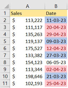
With the second formula, we have made our rule static, which will always highlight the dates we set.