Excel offers the condition formatting feature to format a cell or range of cells based on the value.
But there is also a way to format the entire row using a single criterion. This condition can be based on text, number, blank cells, etc. You can even use multiple criteria.
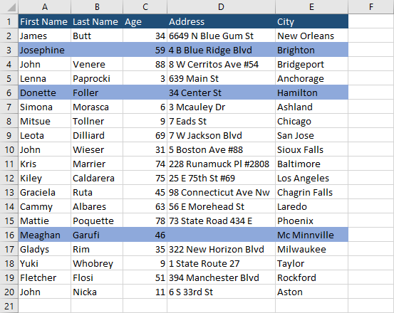
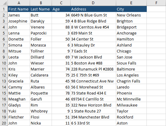
This is an example we are going to use.
Text criteria
The first condition is the text. Here, I’m going to use two examples. In the first one, Excel will highlight the rows in which the values of the cell are exact matches. In the second one, we are going to highlight cells that contain a substring.
Highlight rows (exact match)
In this example, we are going to highlight cells in column A, where the name is “John”.
Select cells from A2 to E20 and navigate to Home >> Styles >> Conditional Formatting >> New Rule.
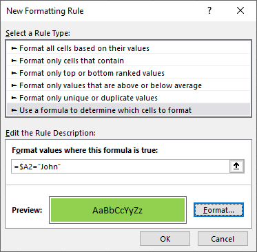
Click, “use a formula to determine which cells to format” and insert the following formula into “Format values where the formula is true”.
|
1 |
=$A2="John" |
Click Format, and choose a color to Fill.
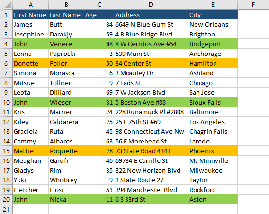
This is how it looks like.
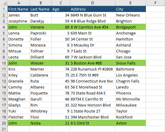
By adding the dollar sign ($) before the cell address we indicated to highlight the entire row and not only the cell where the condition is met.
Highlight rows (contains substring)
In this example, let’s find names that contain a substring “tt”. Use the same options as before, but this time choose different fill and the following formula.
|
1 |
=FIND("tt",$A2) |
And this is our result.
Multiple rules
In Excel, there is a way to add all of these rules at once.
Navigate to Home >> Styles >> Conditional Formatting >> Manage Rules.
Click New Rule, and add all three rules.
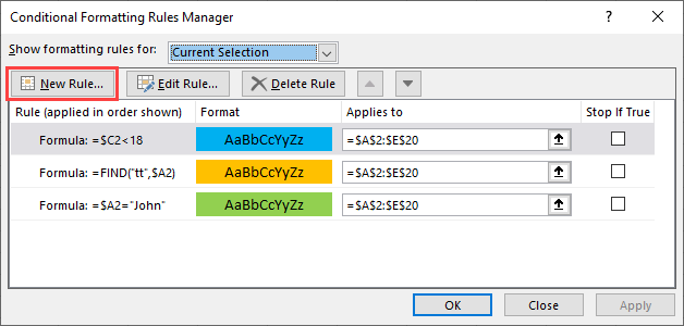
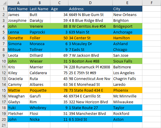
You have to remember that the upper rule has a priority over the rule that is below. That’s why in row 20, it’s highlighted in blue, even that it also met the criterion highlighted in green.
Number criteria
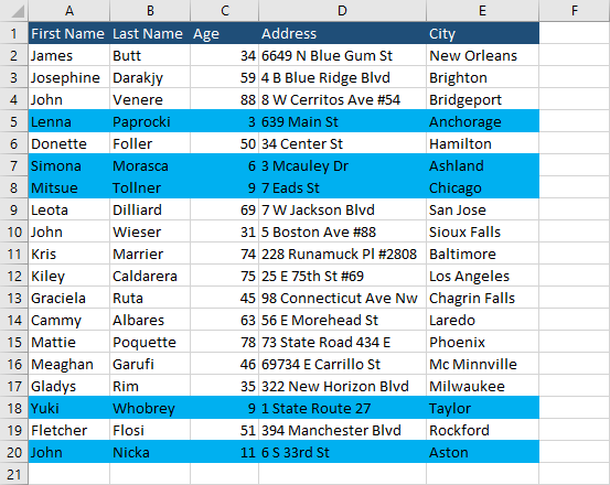
This time, we are going to highlight the entire row based on numbers. We are not going to look for a single number, but numbers that are smaller than 18.
Select cells from A2 to E20, insert new rule and enter the following formula.
|
1 |
=$C2<18 |
Choose a fill and click OK.
Multiple criteria
So far we use a single criterion for each example.
This time, we are going to use two. To do it let’s use AND and OR function.
OR condition
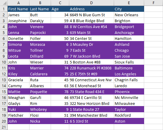
This formula will highlight all rows with people that are not working (below 18 and over 65).
|
1 |
=OR($C2<18,$C2>65) |
Because there is a dark background, in this case, let’s set the font color to white.
This is how it looks like.
AND condition
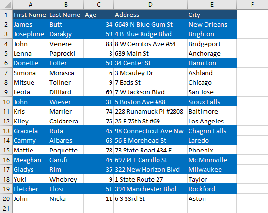
Now, let’s highlight employees (between 18 and 65).
Use this formula.
|
1 |
=AND($C2>18,$C2<65) |
Blank cells
To demonstrate the last example, delete values inside a few cells. In this example, these will be B3, C6, and D16.
Use this formula to check for blank cells.
|
1 |
=COUNTIF($A2:$E2,"")>0 |
This is the result we will get.
