Conditional Formatting is a great tool in Excel for highlighting the data that we want to show and formatting the cells based on certain criteria.
Working with Conditional Formatting, it is important to know the order of the rules, since this is the main factor that determines how these rules are applied to our data.
Excel always applies these rules in the order they appear in the Conditional Formatting Rules Manager, from top to bottom. In the example below, we will show how this works, and how to change the rules order.
Conditional Formatting in Example
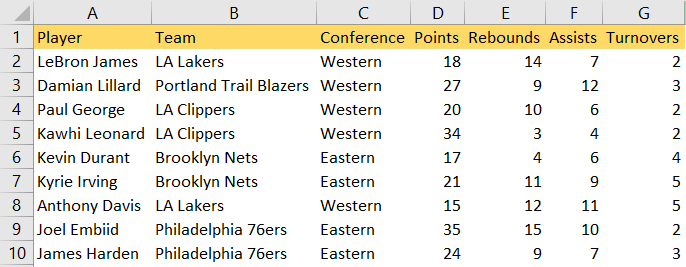
For our example, we will use the list of NBA players, and their statistics from several categories (points, rebounds, assists, and turnovers) from one playing night:
First thing, we need to define our rules. Our first rule will be to color all the data in column D that are between 20 and 30 in yellow.
We will do this by selecting the data in column D, then going to the Home tab >> Conditional Formatting >> Highlight Cells Rules >> Between:
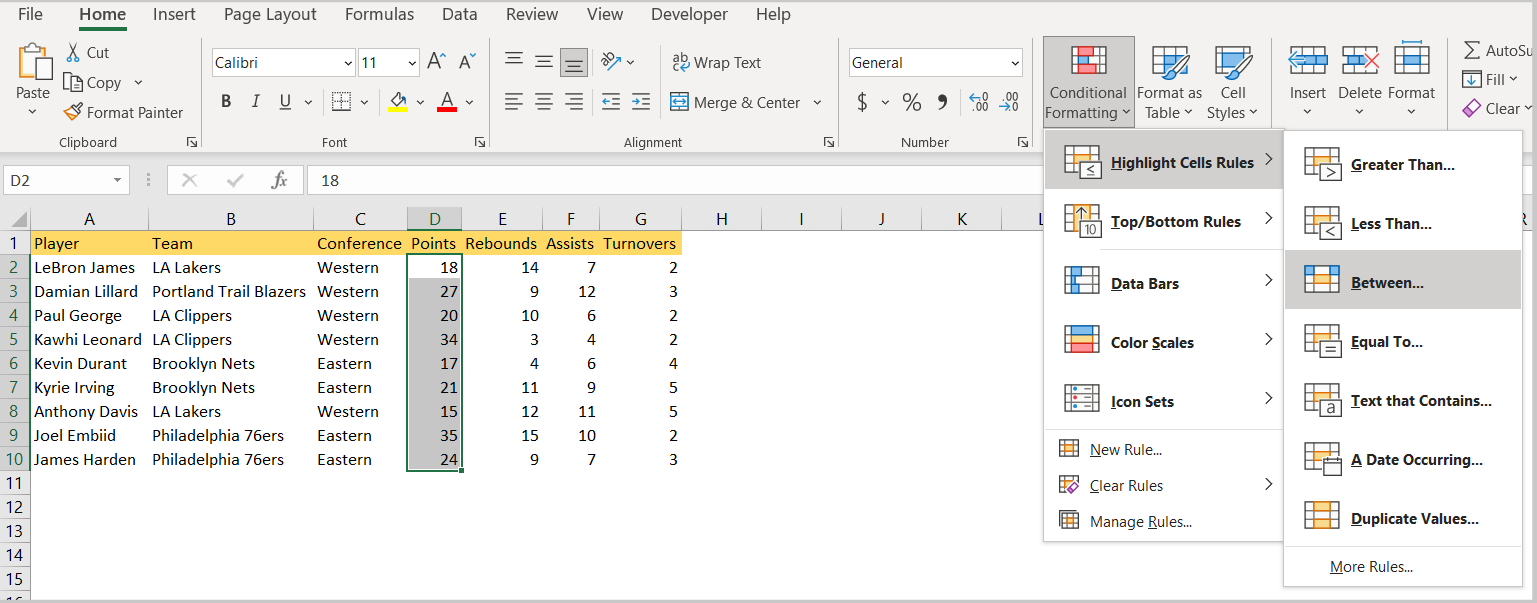
On the window that appears, we will choose 20 and 30 as limits under Format cells that are BETWEEN, and Yellow Fill with Dark Yellow Text under with:

When we click OK, these formatting changes will be applied.
Let’s say that we now want to do another formatting and that we want to highlight every cell in column D with more than 25 points in red. To do this, we will basically use the same approach- highlight the cells in column D, go to the Home tab, choose Conditional Formatting >> Highlight Cells Rules >> Greater Than:
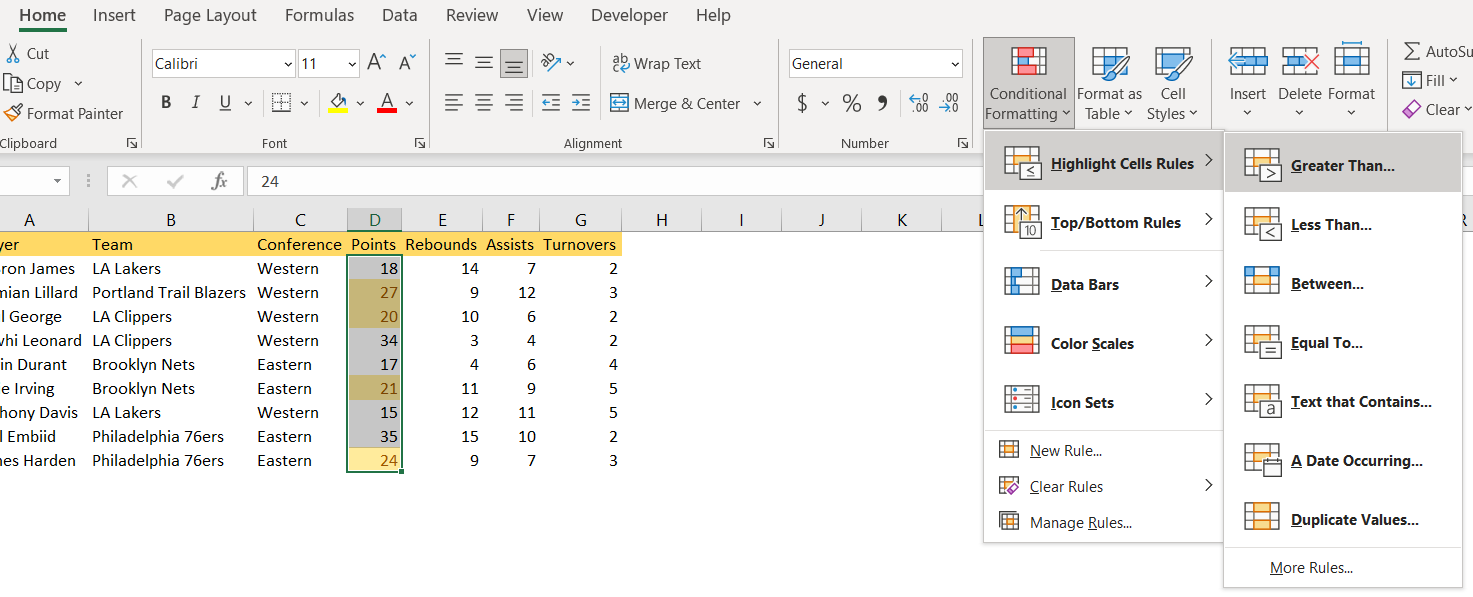
In the window that appears, we will insert number 25 under Format cells that are GREATER THAN, and choose to fill these numbers with Light Red Fill with Dark Red Text:
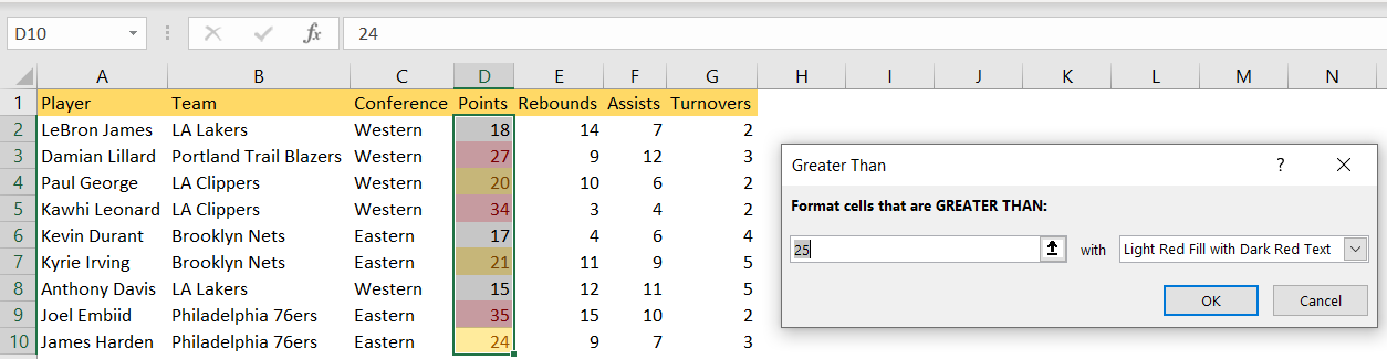
In the table above, we can see the issue that we have at this moment. We have one player- Damian Lillard– located in row number 3, who falls into both categories, since his number of points (27), is both between 20 and 30, and higher than 25.
At this point, the cell that indicates his points is highlighted in a light red fill. But what if we wanted to change that, to be the light yellow color, which is defined in the first rule that we made?
Conditional Formatting Order in Excel
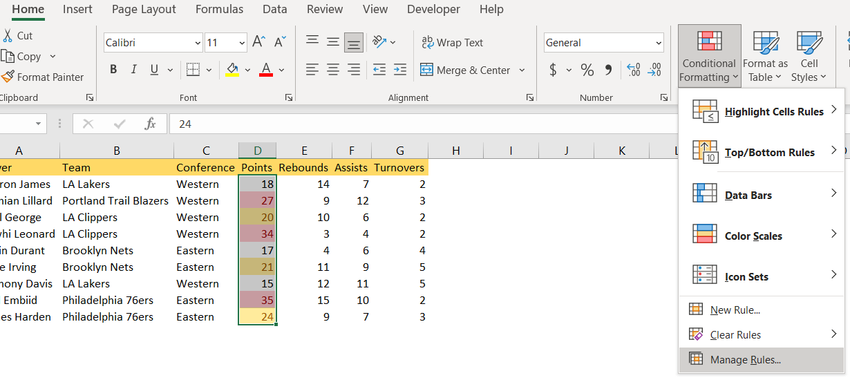
To change the order of the conditions for formatting that we defined, we need to follow a similar path as with setting the rules. We go to the Home tab, then choose Conditional Formatting, and choose Manage Rules from the dropdown menu:
When we click on Manage Rules, we open the Conditional Formatting Rules Manages, which will allow us to move a certain rule up or down in the list. To do this, we need to select the rule, and then click the “Up” or “Down” arrow, which is located on the right side of this dialog box:
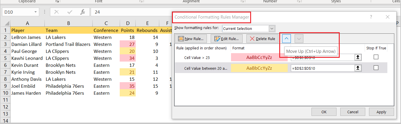
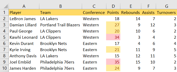
With these arrows, we can manipulate which rule will be looked at first. We will move the rule that we created first in the first place, click OK, and we will have Damian Lillard’s points figure painted in yellow:
As seen in the window in the Rules Manager, we can also Edit or Delete defined rules from this window. In our case, changing the order of our rules gives us control of the way our data is formatted.