Conditional formatting is very useful if you have to deal with thousands of rows of data. With conditional formatting, you can visualize trends and patterns much more quickly than without it.
You can find this feature by navigating to Home >> Styles >> Conditional Formatting.
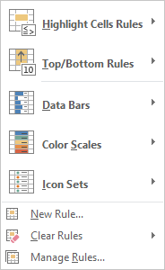
The five top icons are quick rules with suboptions, but if you want to have bigger control over them, you have to create a new rule.
Conditional formatting rules
After you click on the New Rule button, you get access to six types of rules.
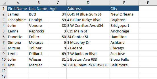
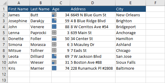
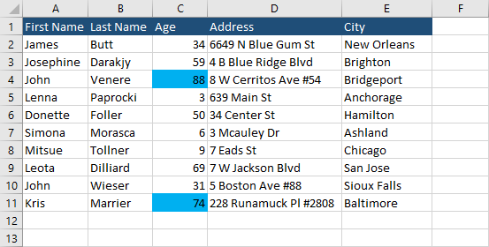
In this tutorial, I’m going to explain each of these rule types. Here’s an example, we are going to use.
Format all cells based on their values
With this rule, you can create conditional formatting for data bars, color schemes, and icons sets.
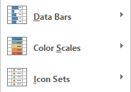
The difference is that when you create a New Rule, you have much more control over the way how this formatting is displayed.
2 and 3 color scales
If it’s a color scale, you can choose exactly which color you want to use for minimum, midpoint, and maximum values. You can also type, such as:
- Lowest value
- Highest value
- Number
- Percent
- Formula
- Percentile
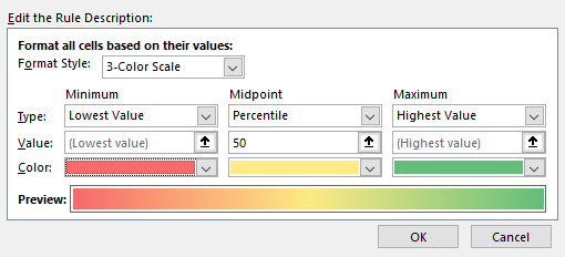
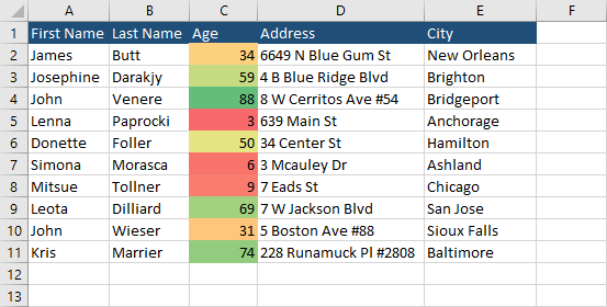
This is the default result without any changes.
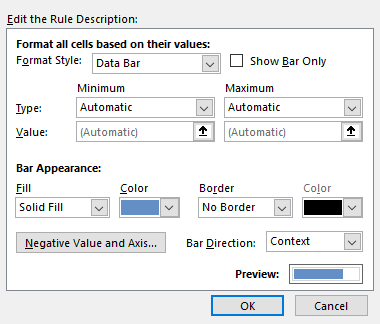
Data Bar
In this format style, you have options to choose between solid fill and gradient, decide whether you want to display bars with the border or without, and choose the option to show bars with values or without values.
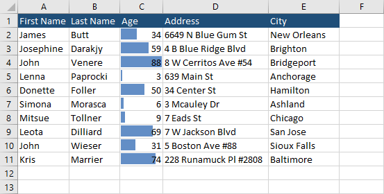
This is the result of the data bar.
Icon Sets
This rule uses icons. Excel offers a list of different icon sets. Values are divided between three to five icons.
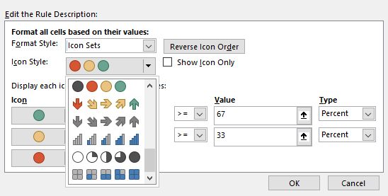
This is one of the sets.
Format only cells that contain
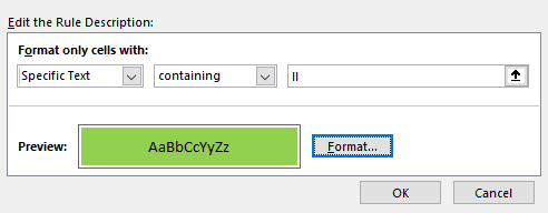
In this rule, you can search for blank cells, errors, dates, and specific text.
If you choose one of these options, for example, specific text, there will be additional options.
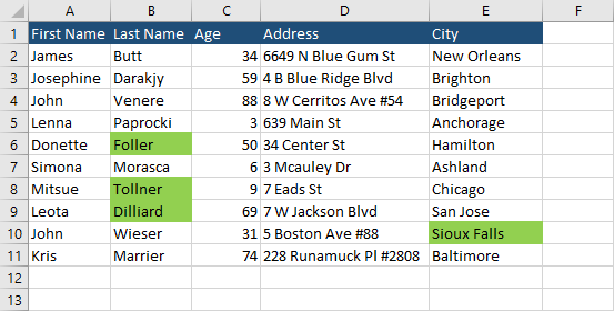
Let’s choose “containing” and insert “ll” to find cells containing this text.
Before you click OK, click the Format button and choose a fill.
I selected the whole table and got this result.
Format only top or bottom-ranked values
This rule allows you to choose the number or percentage of top or bottom values.
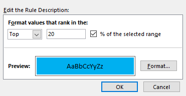
This rule will format 20 percent of the top values. In our example, it will 2 values, because we have 10 numbers.
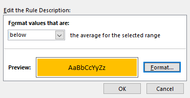
Format only values that are above or below average
Here, you can display values that are above or below average.
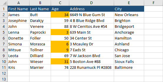
This is the result.
There are more options when it comes to averages, such as 1, 2, and 3 standard deviations.
Format only unique or duplicate values
This rule by default returns duplicate values. You can also change it to unique.
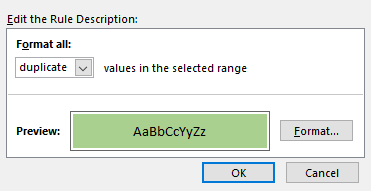
In this example, we are going to leave formatting for duplicate values.
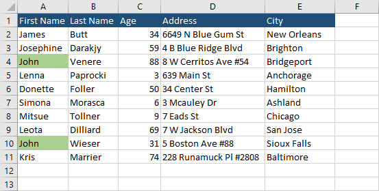
We have a duplicate in our example, so Excel formatted both of them.
Use a formula to determine which cells to format
With the last option, you can write a formula to use formatting for a specific case. You can learn more about this option in the article about formatting the entire row with formula formatting.
