Conditional Formatting in Excel with TRUE and FALSE Values

The advantages and the beauty of using Conditional Formatting have been shown in several examples.

We can use it to mark the things in our column or table that we want to highlight. In the example below, we will show how can we use it to highlight the True and False values.

Formatting True and False Values

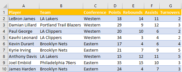
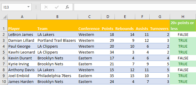
First thing first, we need to create a table with our data. We will use our typical table with NBA players, and their statistical data from one night of basketball, which includes points, rebounds, assists, and turnovers:

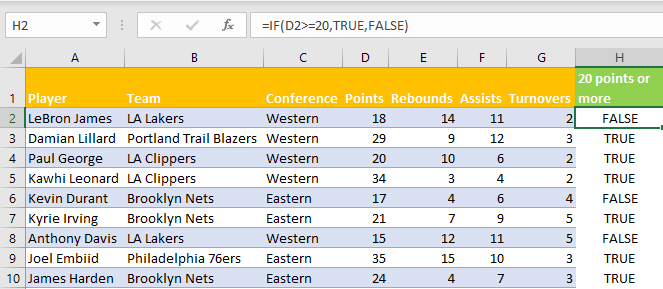
We will define that in column H (the new column that we will create), every row where players scored 20 or more points is TRUE, while other rows will be marked as FALSE.

The formula in cell H2 will be:

We will drag our formula till the end of the table, and our data will look like this:

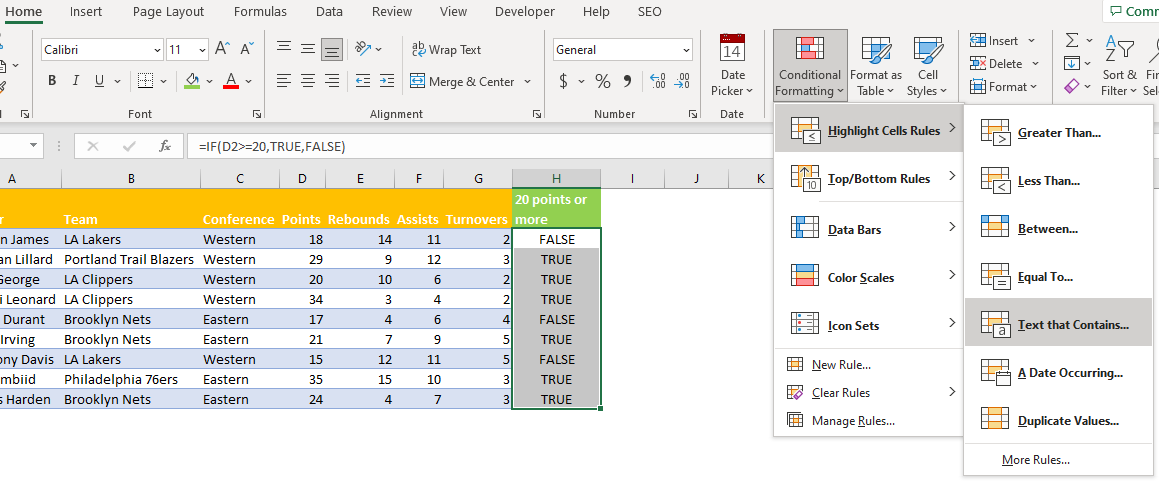
Now, we need to format the column based on these values. We will select range H2:H10, and then go to the Home tab, and after that Styles >> Conditional Formatting >> Highlight Cells Rules >> Text that Contains:

On the window that appears, we will insert TRUE in Format cells that contain the text part, and choose any option for a format that we like. In our case, it will be one of the custom-made options: Green Fill with Dark Green Text:

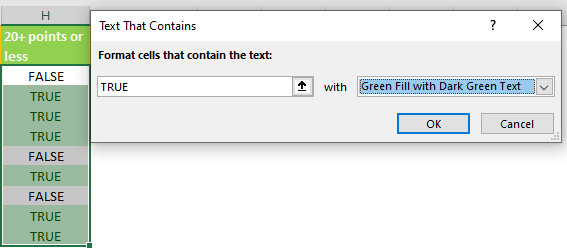
It is noticeable that, even before we click OK, we will have a preview of how our formatting will look like. We will click OK and will have the data same as in the preview:

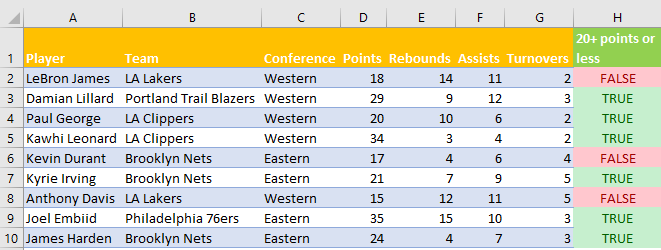
We will do the same thing for values FALSE, but choose Red color as an option:

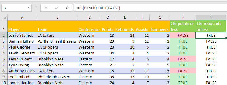
For the next step, we will create the same logic for rebounds in column I, marking rows with equal and more than 10 rebounds as TRUE, and the rest as FALSE. The formula in cell I2 will be:

We will drag the formula till the end of the table again, and get the following results:

We will select the range I2:I10, and then go to Home tab >> Styles >> Conditional Formatting >> New Rule:

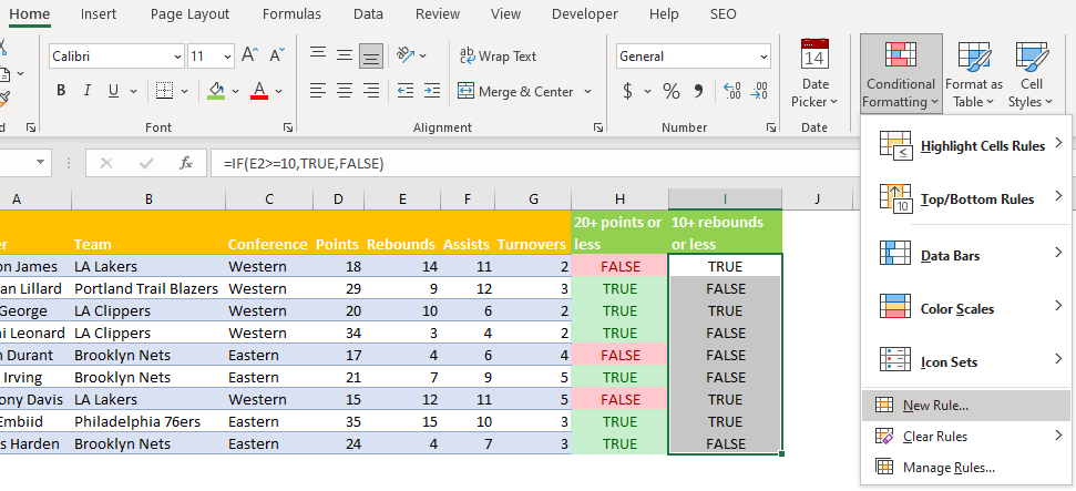
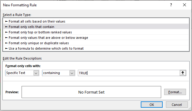
In the window that appears, we will choose several options. Under the Select a Rule Type, we will choose the second option: Format only cells that contain.

In the Edit the Rule Description part of the window, we will choose Specific Text and containing word TRUE in a dropdown under Format only cells with:

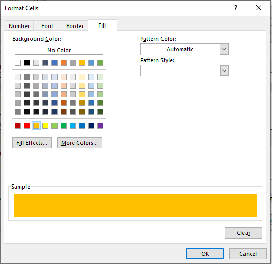
For the last part, we need to choose our formatting. We will click on Format, choose the Fill tab, and then choose the background color (orange in our case):

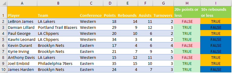
When we click OK, this will be the result in our table:

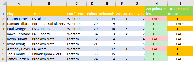
We will do the same thing for FALSE values, and choose blue as a background color for these values. This is our result: