Working with Excel can help us gather and present our data in virtually every way possible. Users are often confused and get stuck when dealing with dates, as they can be tricky to handle and understand.
In the example below, we will show how to deal with one of these issues, and that would be how to convert monthly data to quarterly data. There are several ways to do this, and they can be summarized in three basic ways: using Grouping, using Vlookup, and using Formulas.
Grouping
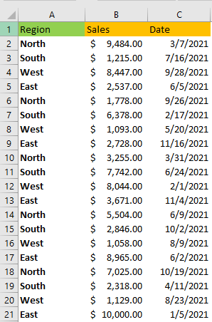
For our example, we will use the sales figures from different regions achieved on different dates:
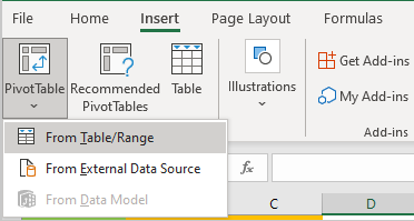
The first thing we need to do is to group the sales figures in months, and then in quarters. To do so, we will select our data, and create a Pivot Table by going to Insert >> Tables >> From Table/Range:
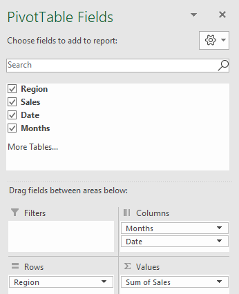
We will click OK in the window that appears, and in the new Pivot Table that appears, we will put Region in Rows, Sum of Sales in Values, and Date in Columns. When we do that Excel will automatically add Months to our dates, which is pretty convenient:
This is what our table looks like after these changes:
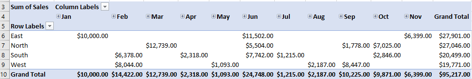
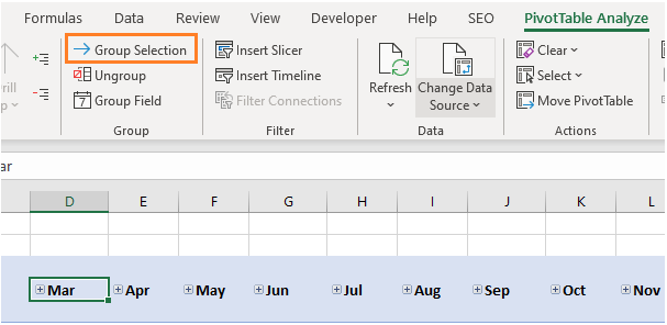
Now, we have our data in months, but we need to change it to quarterly data. What Excel did automatically for us, we now need to do manually. We need to click on the Column Labels toolbar, and then go to PivotTable Analyze >> Group >> Group Selection:
In the window that appears, we can see a couple of possibilities:
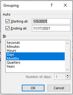
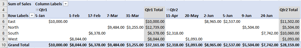
As we want to encompass the whole year of 2021, we will change the starting and end date to 1/1/2021 and 12/31/2021, respectfully. After that, we can replace Months with Quarters in the table. We will do just that and our window will be as follows:
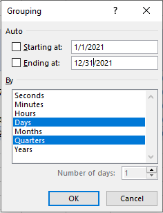
When we click OK, we will have our sales data presented in the quarterly form in our Pivot Table:
Vlookup
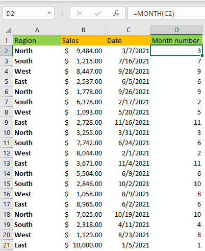
There is also a great and neat way to get the quarterly data with Vlookup. We first need to extract the month number from our dates, and we will do that by entering the following formula in cell D2:
|
1 |
=MONTH(C2) |
In column C the full dates are located. We will drag the formula to the end of our range, and this is what we will end up with:
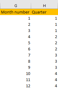
Now we need another table, in which we will connect the months with quarters. In this table, we will have number one for the first three months, number two for the next three, three for months numbered as seventh, eighth, and ninth, and four for the last three months:
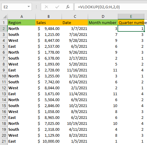
The last thing we need to do is to use Vlookup to connect the dots. The formula will be inserted in column E, and this is what it will look like in cell E2:
|
1 |
=VLOOKUP(D2,G:H,2,0) |
Our lookup value is a month when the sales were achieved, and the lookup range is the table that converts months into quarters. This is the result:
Formulas
What we did above with Vlookup, could be even easier with the IF formula. We will insert the formula in column F, and the formula in cell F2 will be as follows:
|
1 |
=IF(D2<=3,1,IF(AND(D2>3,D2<=6),2,IF(AND(D2>6,D2<=9),3,IF(AND(D2>9,D2<=12),4)))) |
This formula defines the same thing as the Vlookup but in one line. It searches for a value of a particular month and then it groups that value to a particular quarter.
This is the result we end up with when we drag this formula to the end of our range:
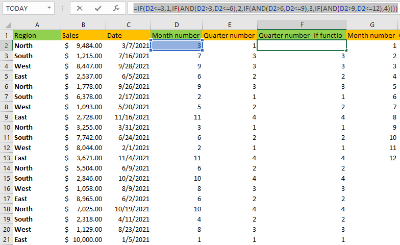
The results in columns E and F are the same. To find the sum or average of a particular quarter, we can easily filter our data and choose a particular quarter.
There is, however, one formula that can encompass a lot of the things that have been done above. It is not just one formula, but rather several of them joined together.
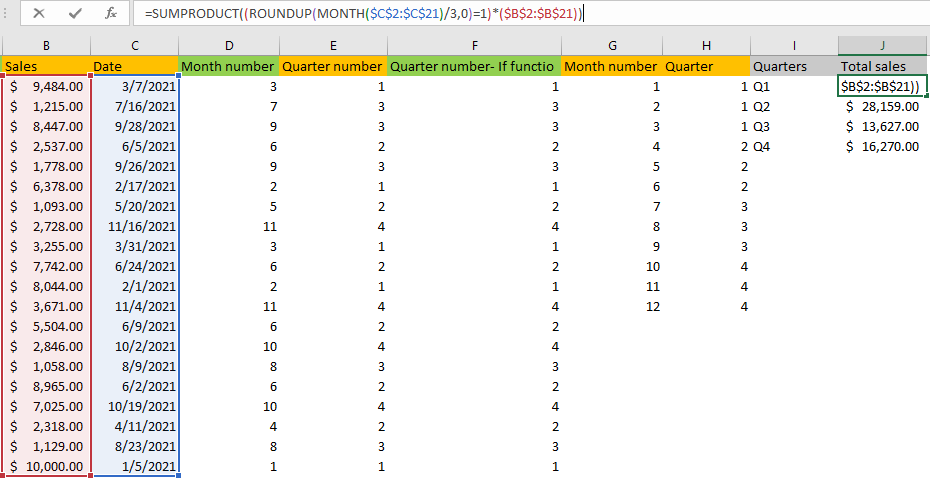
We will insert the formula in column J and then explain it. The formula in cell J2 is as follows:
|
1 |
=SUMPRODUCT((ROUNDUP(MONTH($C$2:$C$21)/3,0)=1)*($B$2:$B$21)) |
Starting from the middle of the formula, we will extract the month from our dates (MONTH formula), which are located in column C. Then the month number for every date will be divided by 3, and the ROUNDUP formula will find every result of this division that is close to 1 (rounded up, so that means months 1,2, and 3, i.e. January, February, and March). As the result, we will end up with a bunch of 0 and 1 in our array. SUMPRODUCT formula is used to multiply all the 1 that we find with the actual sales from that month.
We will lock the range for dates and for sales figures (by using F4 on our keyboard) and then drag the formula to the cell J5. To get results for quarter two we have to change the number after the equation sign, so the formula will be:
|
1 |
=SUMPRODUCT((ROUNDUP(MONTH($C$2:$C$21)/3,0)=2)*($B$2:$B$21)) |
And we will do the same thing for quarters number three and number four, by inserting number 3 and number 4, respectively. This is our result: