Count Occurrence of a Word in a Range in Excel

There are a lot of times when we need to count things in Excel. Excel has many options and functions to help us with this.

In the text below, we will show how can you count the occurrence of a certain word in a range, whether it be a string or a column.

Column with Formula

Counting the occurrence of a word in a column is fairly simple to do and can be done with the formula COUNTIF. This formula does just what you presume- it shows the count in the range based on the criteria that we add.

It has two parameters:

• Range: From where we want to extract the data.
• Criteria: What are the criteria that need to be satisfied so that our range is counted.

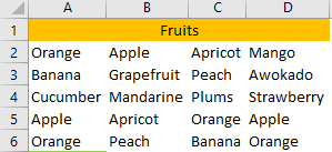
We will use a simple table of different fruits for our example:

If we want to count the number of times that the word “Orange” appears in column A, we will input the following formula in cell A7:

We will get the following result:

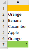
The word „Orange“appears two times in the first column, which is shown in the table above as well.

Multiple Columns with Formula

If we want to count the occurrence of the word „Orange“ in our table as a whole, there is no reason why we should not use the same function again.

Of course, we have to include all of our cells in our formula range now, not just the ones from the first column.

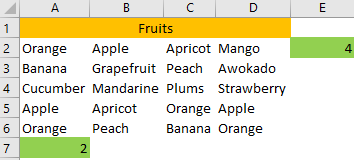
We will place our formula in E2 cell and the formula will be:

The result is four, which means that the word “Orange” is occurring four times in our range.

Column with Pivot Table

There is also a neat way in which we can count the occurrence of a word with Pivot Table. To do this, we will unmerge the first row and then create four different columns (Fruits 1, Fruits 2, Fruits 3, and Fruits 4).

Then, we have to select our range, then go to Insert >> Tables >> Pivot Table.

When we create the table we will put Fruits 1 the Rows Field and Fruits 1 in values as well.

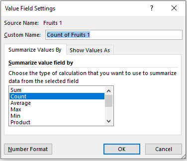
We will choose Count in Value Field Settings:

Our table looks like this:

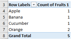
We can see the occurrence of every word in our range.

Cell with Formula

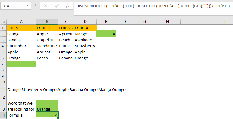
For the last example, we will write the various fruits in the same cell. We will input them in a cell A11, and our sentence will look like this:

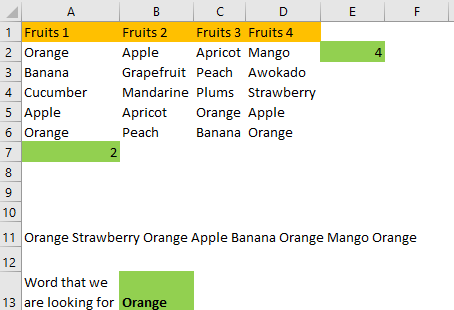
The word that we will look for will be, obviously, “Orange”.

The formula that we have to input the find the occurrence of the word “Orange” in our range will be:

The basic idea of this formula is to count a number of that word in a specific range and to then divide it by the length of the word.

Orange is appearing four times in a range, so its total length is 24 (4×6).

First, we will explain all of these functions as follows:

SUMPRODUCT– this function, as its name suggests, gives us the sum of the products for our range.

LEN– is short of length, and this function returns us the length of a string.

SUBSTITUTE– this one is pretty self-exploratory. It substitutes one or more instances of a given string.

UPPER- this function makes all the letters in our text string as upper letters, thus making sure that our string is not case sensitive.

These functions are used in the upper formula as follows:

It returns the count of characters in our range, which is, in our case, 57.

Substitute replaces a word in B13 (which we made to be a word “Orange”) with the empty sign- ““. Then LEN functions come into place. It returns the count of characters after we did the substitution. We will get 33 as a result of this.

It returns the length of a word in B13 which is number 6 (for the word “Orange”).

Finally, we have the SUMPRODUCT formula that takes place. When we did all the calculations, we are left with:

This will give us number 4, of course.