Excel has so many powerful options that can be utilized, and we have described a lot of them so far.
If we want to find out the number of rows in our table, there are many ways to do so. In the text below, we are going to show some of the easiest ones.
Count Rows with Formula
For the example, we will use a simple list of different fruits.
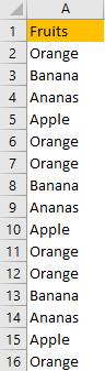
Now, there is no need to say that, for this example, it is pretty easy to count the rows, as their numbers are shown on the left side.
This example is simplified but the formula can be used in a table of any kind.
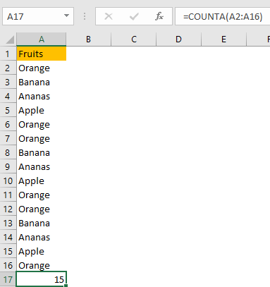
We will input a formula in cell A17. The formula is as follows:
|
1 |
=COUNTA(A2:A16) |
Keep in mind that we did not want to include the first row from the count.
COUNTA formula has the following syntax:
|
1 |
=COUNTA (value1, [value2], ...) |
It has two arguments:
- value1 – An item, cell reference, or range.
- value2 – [optional] An item, cell reference, or range.
This formula returns the count of cells in our range that contain either text, number, logical value, error value, or any value that is not empty.
Our value is our range, and we got the result as follows:
If we had empty cells in our range, we would use a different formula- COUNTBLANK. This formula counts only empty cells.
So, if we had empty cells in our range, we could use this formula.
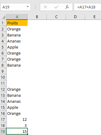
We will delete a couple of entries in our table, keep our existing formula, but will add COUNTBLANK beneath.
Finally, we will add these two numbers together, and get the number of rows in our table:
Count Rows with VBA
To count the rows with VBA code, you have to open the VBA editor either by going to Developers tab >> Code >> Macros or simply by clicking ALT+F11, and entering the following code:
|
1 2 3 4 5 6 7 |
Sub CountRows() Dim final_row As Long final_row = Cells(Rows.Count, 1).End(xlUp).Row MsgBox (final_row) End Sub |
For this code, we first declared a variable final_row to be the Long type. This type is used when working with a large set of numbers.
Rows.Count gives us the number of rows in a worksheet. Excel checks each value, from our final row by moving up.
For the final part, we wanted that our code to print out the message of how many rows are in our table, so we get this message after we run our code:
If we want to exclude the first row, we can add the following part in our code, right after the line of code in which we declared our variable:
|
1 |
final_row = final_row – 1 |
Remember that this code takes even empty cells into the consideration.
There is a problem that we could if using the code above for different tables. We could have some columns that contain more rows than others, like in the picture below:
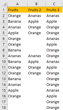
If we execute our code now, the result will be number 16 again, which is not the correct number as we have 18 rows in column C. We have to change our code a little bit:
|
1 2 3 4 5 |
Sub CountRows2() Dim final_row As Long final_row = Cells.Find(What:="*", SearchDirection:=xlPrevious).Row MsgBox (final_row) End Sub |
The second line in the code is now looking for any data in our table. The xlPrevious indicates Excel to search for a value in the last Excel sell and then move from right to left from the last row to the first row until it finds a non-blank cell.
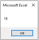
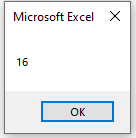
When we execute it, we will have the correct result, which is 18:
The second line in the code is now looking for any data in our table. The xlPrevious indicates Excel to search for a value in the last Excel sell and then move from right to left from the last row to the first row until it finds a non-blank cell.
When we execute it, we will have the correct result, which is 18: