Create a Scrolling Chart in Excel

When we create a chart based on a big dataset that does not fit in the Excel Window, Excel cuts off some values. We can prevent this by creating a scrolling chart.

A scrolling chart has a scroll bar that allows us to scroll through and view all the data points.

Step 1: Create a default chart

We are going to demonstrate how to create a scrolling chart in Excel using the following dataset:

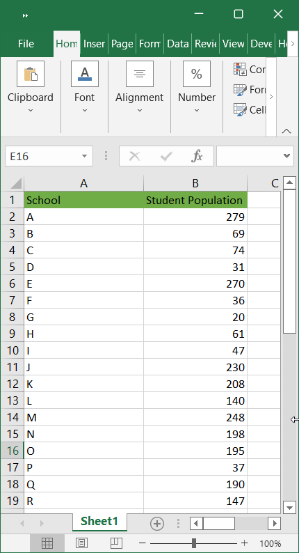
The first step is to create a default chart. We are not going to adjust its data source in the end but for now, it helps us to see how the chart window adjusts to accommodate the data points.

We use the following steps to create the chart:

1. Insert a chart based on the dataset by selecting a cell in the dataset and then clicking Insert >> Charts >> Recommended Charts.

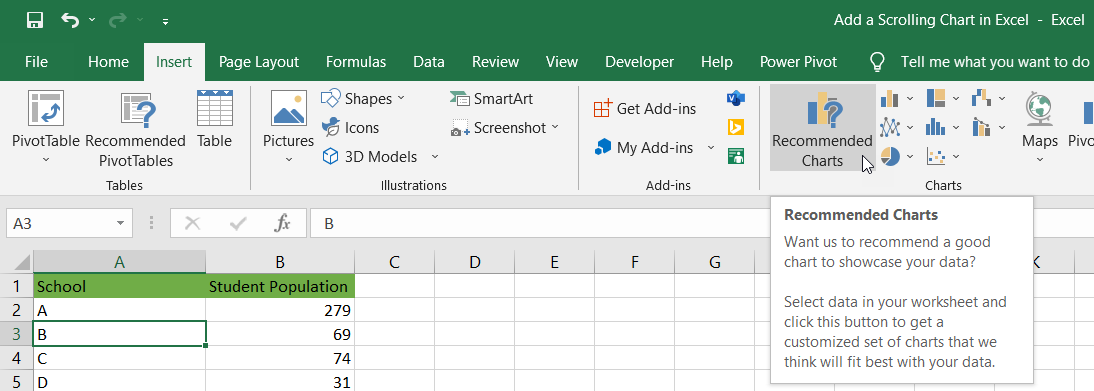
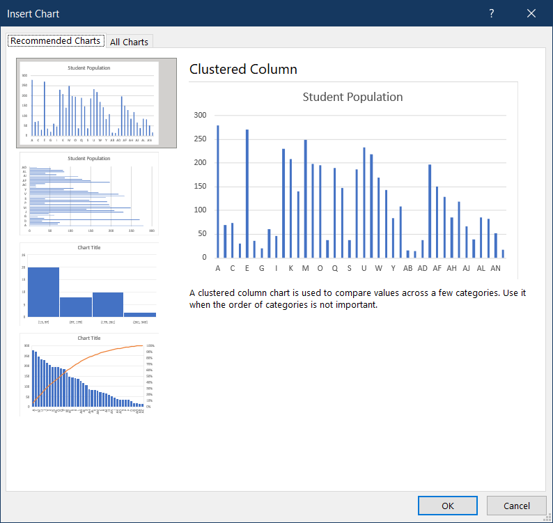
2. In the Insert Chart dialog box, review the recommended chart to check if it is appropriate and click OK to insert it. In this case, we insert the Clustered Column chart.

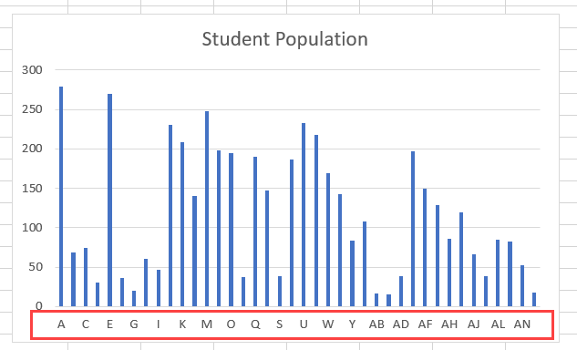
The chart is inserted into the worksheet. Some data points have been cut off by Excel, for example, data points B and D.

Step 2: Insert the scroll bar control and adjust its settings

We add the Scroll Bar control to the worksheet by using the following steps:

1. Click Developer >> Controls >> Insert >> Scroll Bar to insert a scroll bar into the worksheet.

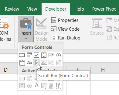
Note: If we do not see the Developer Tab on the Ribbon, we can enable it by clicking File >> Options >> Customize Ribbon and selecting Developer in the Main Tabs box on the right of the Excel Options dialog box.

2. Drag the mouse to draw the scroll bar control on the worksheet and then right-click it and select Format Control on the shortcut menu.

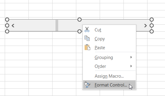
Note: Where we position the control is not important now because we will move it later.

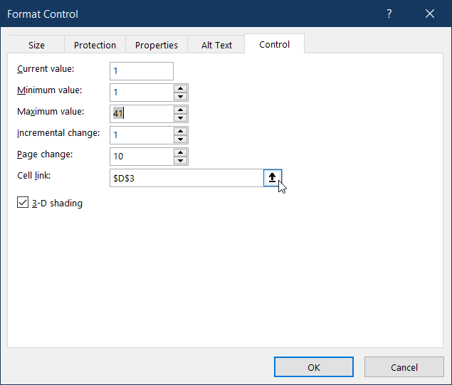
3. In the Control tab of the Format Object dialog box, specify the Minimum value and Maximum value of data points to display in the chart as appropriate. Click the up arrow in the Cell link box and select a cell to which we want to link the scroll bar and then click OK.

Explanation of the settings

• Current value. This is the control’s current value that corresponds to the current position of the scroll box in the scroll bar, 1 being the anchoring or initial value of the control.
• Minimum value. This is the lowest value that a user can specify by positioning the scroll box to the left end of the horizontal scroll bar.
• Maximum value. This is the highest value that a user can specify by positioning the scroll box to the right end of the horizontal scroll bar. In this case, it is 41 because this is the total number of records in our data range.
• Incremental change. This is the amount the value increases or decreases and how far the scroll box moves when the arrows at each end of the scroll bar are clicked.
• Page Change. This is the amount the value increases or decreases and how far the scroll box moves when we click the area between the scroll box and either of the arrows at the end of the scroll bar.
• Cell link. This is the cell reference that contains the current position of the scroll box.

Step 3: Define range names for new data source

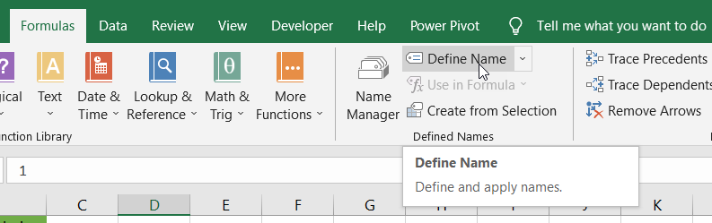
1. To define the name of the first range, select the cell D3 that we specified in the Cell link box and click Formulas >> Defined Names >> Define Name.

2. In the New Name dialog box type School in the Name box and enter the formula in the Refers to box:

3. Click OK to close the dialog box.

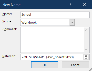
Note: The OFFSET function returns a reference to a range that is a given number of rows and columns from a given reference, Sheet1 is the active worksheet in which that dataset is contained. Cell A2 is the first cell in column A excluding the header. Cell D3 is the linked cell we specified earlier.

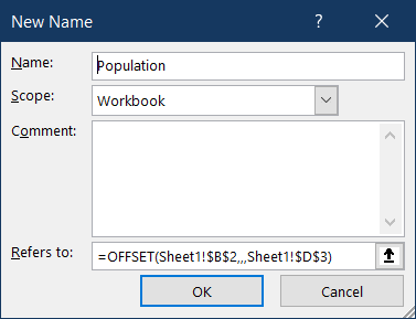
4. To define the name of the second range, select cell D3 again. Then click Formulas >> Defined Names >> Define Name.
5. In the New Name dialog box type Population in the Name box and enter the formula in the Refers to box:

6. Click OK to close the dialog box.

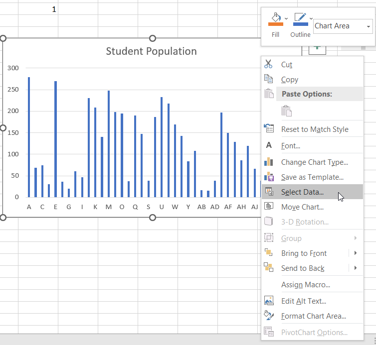
Step 4: Change the data source of the default chart

In this step, we change the data source of the chart we created in step 1 to the new range names we have defined.

We use the following steps:

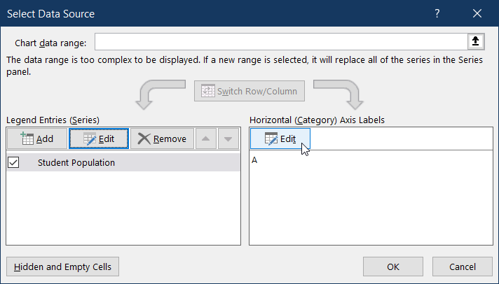
1. Select the chart and right-click it and click Select Data on the shortcut menu.

2. Click Edit in the Select Data Source dialog box.

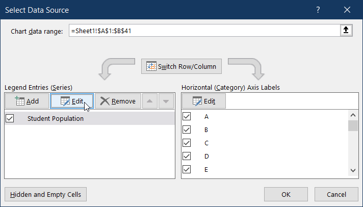
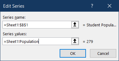
3. In the Edit Series, dialog box enter the formula =Sheet1!$B$1, and enter the formula =Sheet1!Population Series values box and click OK to close the dialog box.

4. In the Select Data Source dialog box, click Edit under the Horizontal (Category) Axis Labels.

5. In the Axis Labels dialog box enter the formula =Sheet1!School. Click OK to close the dialog box.

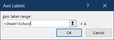
6. Click OK to close the Select Data Source dialog box.

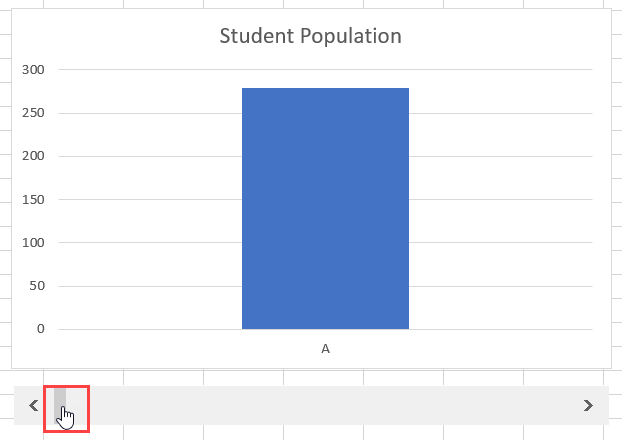
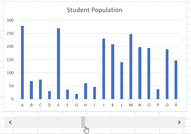
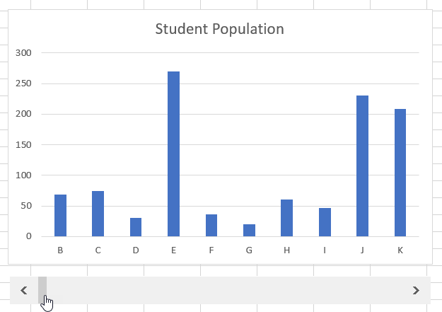
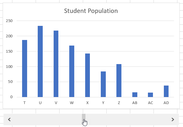
The scroll bar is now added to the chart. We can test it by dragging the scroll box to the left and right and seeing the chart adjust accordingly as in the following screenshots.

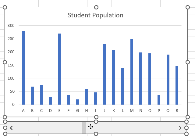
7. To combine the chart and the scroll bar, select the scroll bar and drag it to a position close to the chart. Hold down the Ctrl key and select the scroll bar and then the chart.

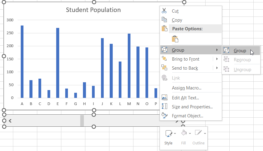
8. Right-click the selection and click Group on the shortcut menu.

Step 5: Adjust and refine the scrolling chart

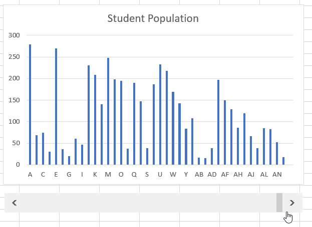
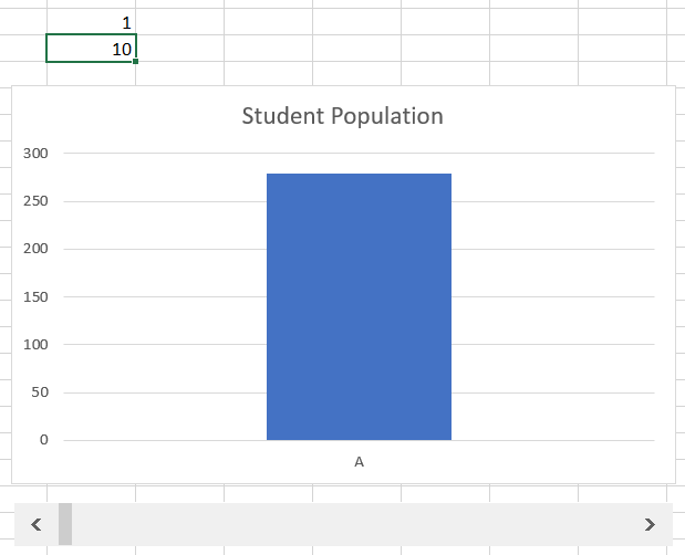
With the scroll bar we have created, when we drag the scroll box to the maximum, we notice that Excel cuts off some data points.

We can fix this problem by setting the number of data points to be displayed at any given time. In this case, we want the number to be 10.

We have copied our scrolling chart to Sheet2 and made the necessary adjustments so we can demonstrate how this can be achieved. All the formulas we entered in Sheet1 have been adjusted accordingly.

We use the following steps:

1. Type number 10 in cell D4 as shown below.

2. To edit the named ranges we created, click Formulas >> Defined Names >> Name Manager.

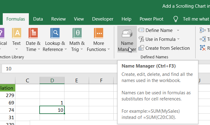
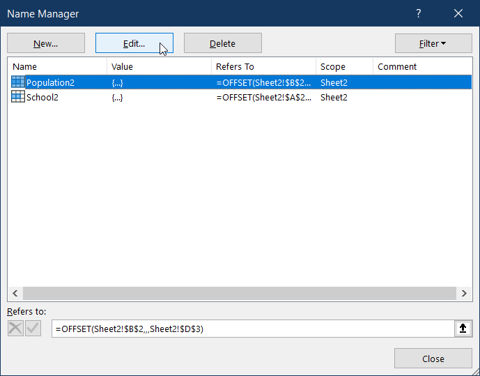
3. In the Name Manager dialog box select Population2 and click Edit.

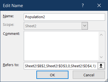
4. In the Edit Name dialog box, in the Refers to box edit the formula to be:

5. Click OK to close the dialog box.

6. In the Name Manager dialog box select School2 and click Edit.
7. In the Edit Name dialog box, in the Refers to box edit the formula to be:

8. Click OK to close the dialog box.
9. Click OK to close the Name Manager dialog box.

The chart adjusts accordingly so that 10 data points are displayed at any given time as shown below:

Conclusion

In this tutorial, we have explored the various steps we need to take to create a scrolling chart in Excel.

A scrolling chart has a scroll bar that allows us to scroll through and view all the data points. This is a very useful feature, especially when dealing with charts that are based on huge datasets.