Create or Remove Hyperlinks in Excel

If you want quick access to associated information on a web page or another file, you can create a hyperlink in a worksheet cell or some chart elements.

In some cases, you may want to remove the hyperlinks from Excel cells so that you remain with only plain text URLs because you don’t want the associated websites to be opened when the cells are selected.

In this tutorial, we will look at 5 ways of creating hyperlinks and 6 ways of removing them.

Create Hyperlinks

We can create hyperlinks to new files, existing files or webpages, specific locations in a workbook, email addresses, or other workbooks located on the intranet or internet.

We will look at the following 5 methods we can use to get this done:

1. Use the Insert Hyperlink dialog box
2. Type in the URL
3. Drag and Drop
4. Use the HYPERLINK function
5. Use Excel SEO add-in

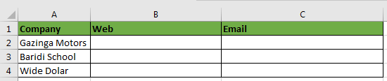
We will use the dataset below to demonstrate how each method works:

Method 1: Use the Insert Hyperlink dialog box

To apply this method we use the following steps:

1. Select Cell B2 in which we want to insert a hyperlink.
2. Launch the Hyperlink dialog box in any of the following ways:

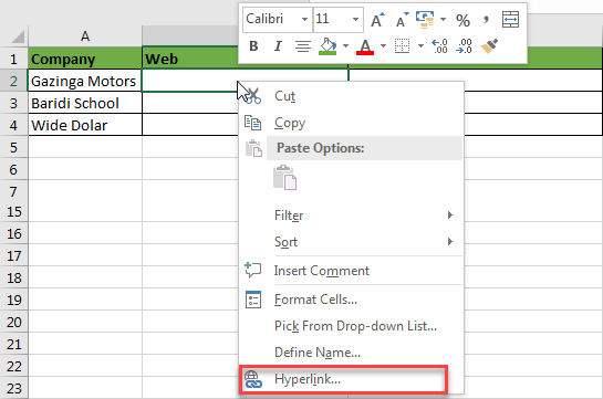
• Right-click the cell B2 and click Link as in the example below:

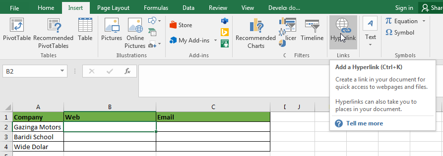
• Select cell B2 and on the Ribbon go to Insert >> Hyperlink:

• Use the keyboard shortcut Ctrl + K.

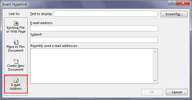
The Insert Hyperlink dialog box will pop up:

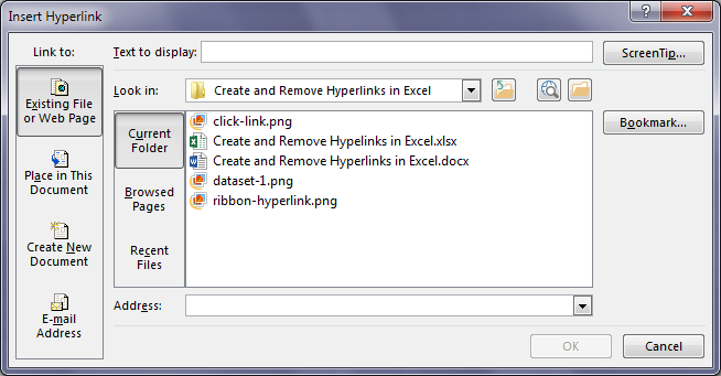
Explanation of the Insert Hyperlink Dialog Box

Text to display box

The “Text to display:” box appears at the top of the dialog box. What is displayed here depends on the contents of the cell where we want to insert a hyperlink.

If the cell contains text, the text will appear in the box. We can edit the text and the revised text will appear in the cell.

If the selected cell is empty the box will also be empty.

If the cell we selected contains a number, the box contents will be dimmed displaying <<Selection in Document>> and we will not be able to edit it. If we want to edit it, we need to close the dialog box, change the numeric value to text, and launch the dialog box again.

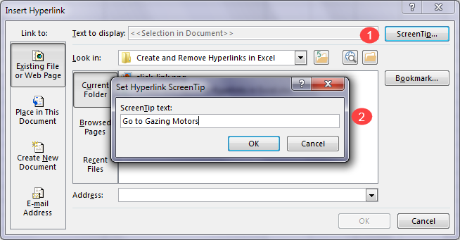
ScreenTip… button

We use this button if we want to add our text for the Screen Tip that appears when we point to the cell that contains a hyperlink.

To add our Screen Tip text, click the ScreenTip… button and type the text in the pop-up box that appears, and then click OK, as in the example below:

Link to Panel

The “Link to” panel is on the left-hand side of the Insert Hyperlink dialog box:

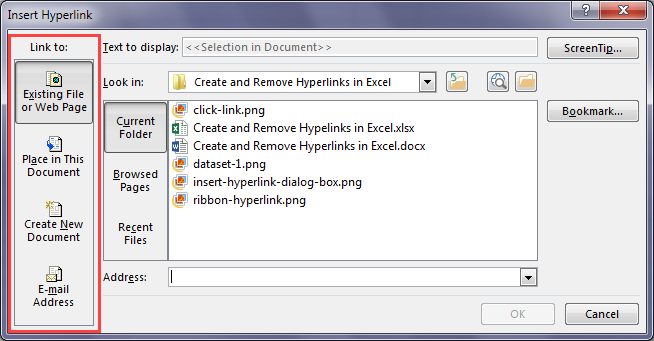
The panel has 4 options:

1. Existing File or Web Page
2. Place in This Document
3. Create New Document
4. E-mail Address

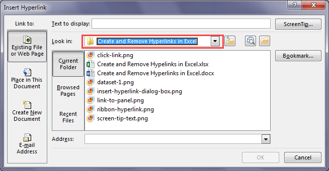
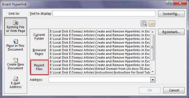
• Link to Existing File or Web Page

We use this option if we want people to open another Excel file, or go to a web page for more information.

To link to an existing file use the folder navigation box to locate and select the file:

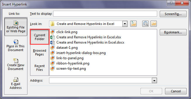
Alternatively, if the file is in the current folder we are working in, we can click on the Current Folder button and then select the file among those listed beside it:

Or if the file we want to link to is one of those we recently worked on, we can locate it by first clicking on the Recent Files button:

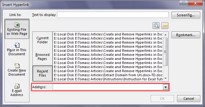
To link to a web page we type its URL in the Address box:

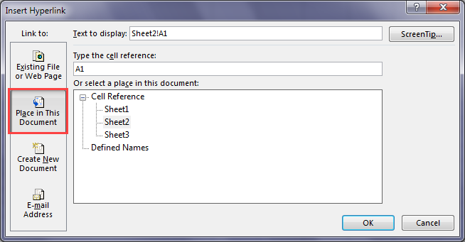
• Link to Place in This Document

We use this option if we want to link to a cell or range in the current worksheet or another worksheet in the current workbook. Change the other settings as needed:

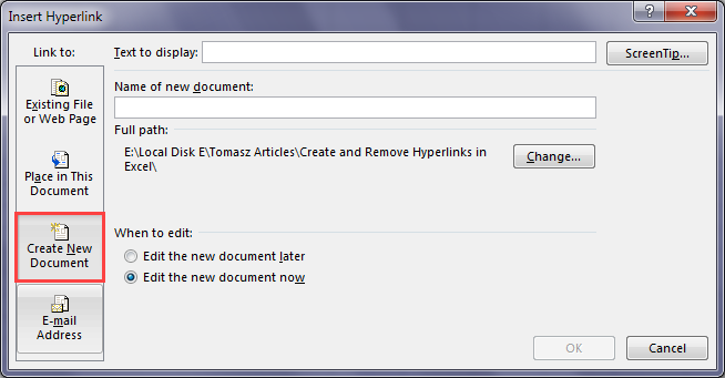
• Link to a New Document

We use this option if we want to link to a new document we want to create. Adjust the other settings as appropriate:

• Link to an E-mail Address

This option is used for linking to an E-mail address. We adjust the other settings as appropriate:

Method 2: Manually type in the URL or Copy and Paste it in

In this method we type the URL in a cell or copy and paste it into the cell and Excel will automatically convert it into a hyperlink.

We use the following steps:

1. Select the cell in which you want to type or paste the hyperlink.
2. Double click the cell or press F2 on the keyboard.
3. Type the URL or Copy and paste it in.
4. Press Enter and Excel will create the hyperlink.

Method 3: Drag and Drop

To apply this method we use the following steps:

1. Ensure the workbook is saved. This method won’t work on a new workbook that is not saved.
2. Select the cell that we want to link to.
3. Point to the border of the cell and Right-click on it.
4. Press the Left Alt key and drag the cell to another sheet’s tab.
5. When the sheet is activated, release the Left Alt key, and drag the cell to the location where you want the hyperlink.
6. Release the right mouse button and click Create Hyperlink Here on the pop-up menu:

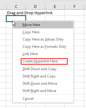
The hyperlink will be created in the selected location.

Method 4: Use the HYPERLINK function

The HYPERLINK function creates a shortcut or a jump that opens a document stored on the hard drive, network server, or on the Internet.

The syntax of the function is:

The link_location is a mandatory argument and can be a place in a document such as a named range, the URL of a web page, or a file on the local hard drive.

The friendly_name argument is optional and is the text that we want in the cell that contains the hyperlink. It can be the company name or a short description. If this is omitted, the URL will be used as a friendly name.

The function can be used to create a link to a website, email, or Excel file.

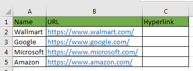
Create a Hyperlink to a Website

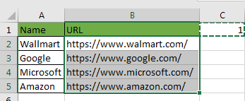
We will use the following example where we have company names in Column A and their URLs in Column B to show how the HYPERLINK function can be used to create hyperlinks in Column C that open the company websites:

To get the result where the friendly name is the company name and the company URL is the link location do the following:

1. Select Cell C2 and enter the formula =HYPERLINK(B2,A2) as follows:

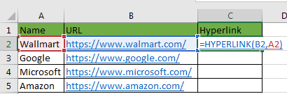
2. Press Enter key and drag down the Fill Handle to copy the formula down the column:

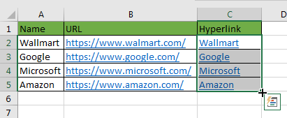
Hyperlinks have been created in Column C.

Create a Hyperlink to an Email

We will use the following example where we have names of company staff in Column A and their email addresses in Column B to show how the HYPERLINK function can be used to create hyperlinks in Column C:

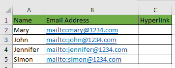
To get the result where the friendly name is the name of the staff and the link location is the email address, do the following:

1. Select Cell C2 and type in the formula =HYPERLINK(B2,A2) as follows:

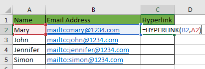
2. Press Enter key and drag down the Fill Handle to copy the formula down the Column C:

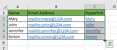
When the hyperlinks are clicked they open the default email program with the email addresses of the staff already filled in the “To” box.

Create a Hyperlink to a range within the same Excel File

The HYPERLINK function can be used to create a link to a range within the same workbook. We achieve this by adding a pound sign (#) at the beginning of the address.

For example, to create a link to Cell B10 in Sheet 1 which contains the budget for the first quarter, we can use the following formula:

Create a Hyperlink to another Excel File in the Same Folder

To create a link to another Excel file that is in the same folder, we use the name of the file as the link location argument for the HYPERLINK function. For example, to create a link to a file called accounts we can use the following formula:

For a file that is in another folder in the same folder use two periods and a backlash at the beginning of the address as follows:

Method 5: Excel SEO Add-in

You can find this free add-in on the main page: officetuts.net.

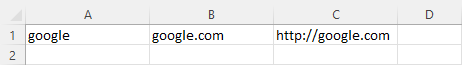
After you install the plugin, Select text to convert to hyperlinks (A1:C1).

Now, click SEO >> Hyperlinks >> Create Hyperlink.

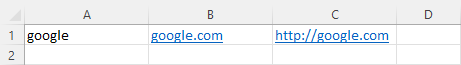
This tool converts to a hyperlink only a string that is recognized as a link, therefore A1 is not converted.

Remove Hyperlinks

We have so looked at methods that we can use to create hyperlinks. But in some cases, we may not want hyperlinks in our Excel files.

We will look at the following methods of removing hyperlinks:

1. Use the shortcut menu
2. Copy and Paste as values
3. Use Paste Special
4. Use the Clear Command
5. Use Excel VBA
6. Use Excel Add-in

Method 1: Use the Shortcut menu

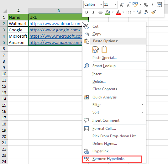
In this method, we first select all the cells that have hyperlinks, right-click and click Remove Hyperlinks from the shortcut menu as follows:

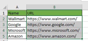
All the hyperlinks are removed:

Method 2: Copy and Paste as values

In this method we do the following steps:

1. Select all the cells that contain hyperlinks and press Ctrl + C to copy them.
2. Select the cells into which we want to copy the cells as Values.
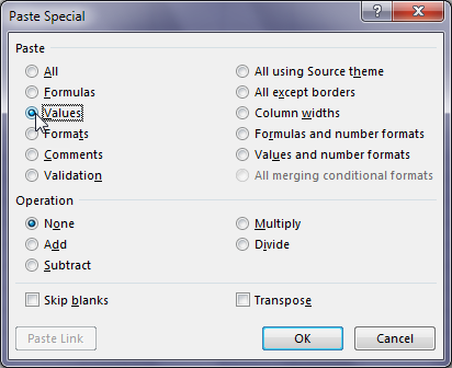
3. Press Ctrl + Alt + V to open the Paste Special dialog box, select Values in the dialog box then press OK:

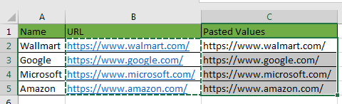
The hyperlinks will be pasted as values and we can now delete the column with hyperlinks because we no longer need it:

Method 3: Use Paste Special and Multiply by 1

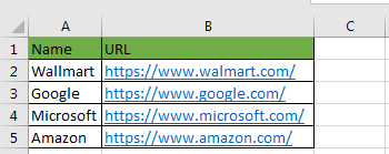
We will use the following dataset to demonstrate how this method can be used:

1. Type the number 1 in Cell C1.
2. Select Cell C1 which contains number 1 and press Ctrl + C to copy it.
3. Select range B2:B5 that has the hyperlinks.
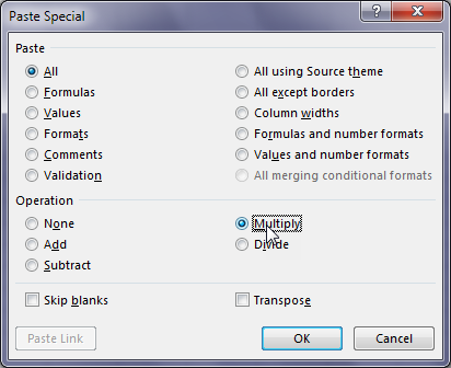
4. Press Ctrl + Alt + V to open the Paste Special dialog box and select Multiply operation, and press OK:

All the hyperlinks are removed:

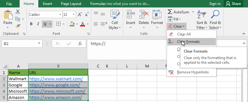
Method 4: Use the Clear Command

In this method we use the following steps:

1. Select the range that contains the hyperlinks.
2. Go to Home >> Editing >> Clear >> Clear Formats:

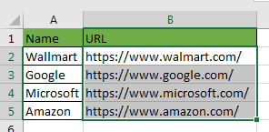
All the hyperlinks plus other formats are removed:

Method 5: Use Excel VBA

If we want to remove hyperlinks from selected cells:

1. Press Alt + F11 to open the Visual Basic Editor.
2. Create a new module and type in the following code:

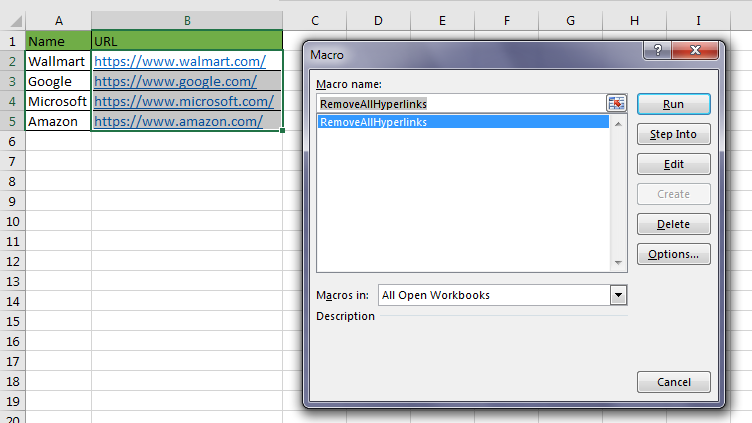
1. Press Alt + F11 to switch back to the active sheet.
2. Press Alt + F8 to open the Macro dialog box, select the RemoveAllHypelinks macro and click Run:

All hyperlinks will be removed from the selected cells.

If we want to remove all hyperlinks from the active sheet we will need to modify the code as follows:

Method 6: Use Excel Add-in

In a similar way to creating hyperlinks with a help of this add-in, you can remove it.

Select cells with data (A1:C1). Two of these cells have links and one doesn’t.

Now, click SEO >> Hyperlinks >> Create Hyperlinks.

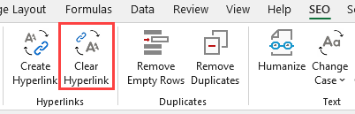
The links are removed, and standard text is left alone.

Conclusion

In Excel, we can create hyperlinks in cells that we can use to go directly to the URL. In this tutorial, we have looked at four different methods that we can use to create hyperlinks in Excel. They are; typing the URLs directly into the cells, using the Insert Hyperlink dialog box, using the drag and drop, and using the HYPERLINK function.

We have also looked at five methods we can use to remove hyperlinks from our Excel files when we no longer need them. These methods are using the shortcut menu, using the Excel VBA, using the Clear Format command, Copy and Paste as Values, and using the Multiply operation on the Paste Special dialog box.

It’s also great to see how custom-made tools and functions can save a lot of work and be advantageous over Excel features and functions.