While working in Excel, you can quickly remove duplicated values when you deal with a few cells. But when you deal with thousands of cells, this is not the best way. It’s not only time-consuming but also error-prone.
That’s why Microsoft gives you a few ways to eliminate duplicates. In this lesson, I’ll show you how you can achieve this using different methods, both the basic ones and the more complicated ones, with the VBA code included.
Highlighting duplicate values using conditional formatting
Conditional formatting is probably the most popular method to distinguish data visually. It can be used to highlight low and high values with different colors. Besides that, you can find here a tool that will help you find duplicated and unique values.
Example:
First, create the following table with names.
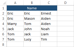
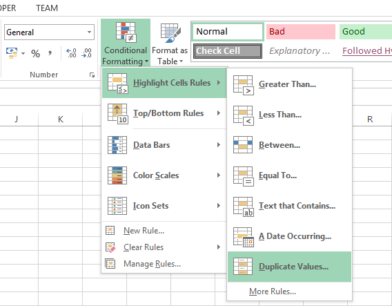
Select all the cells, and choose conditional formatting in HOME >> Styles >> Conditional Formatting >> Highlight Cells Rules >> Duplicate Values.
When you choose this option, a new window will appear.
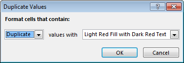
Here, you can choose whether you want to search for duplicate or unique values, and mark them with one of the available formats or even create your own custom format.
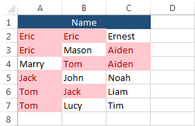
We will get the following result.
Finding duplicate values using DGET
Another way to find duplicates is by using the DGET function. This function is used to retrieve a single record from a database that matches the criteria given in the argument.
This function returns one of three values:
- If no records meet the condition, the function returns the #VALUE! error.
- If one record meets the condition, DGET returns the result.
- If more than one record meets the condition, DGET returns the #NUM! error.
Take a look at the example:
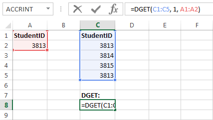
The formula will return StudentID if there is only one StudentID value inside the table. Because there is more than one number 3813 in the C column, the formula will return the #NUM! value.
|
1 |
=DGET(C1:C5, 1, A1:A2) |
Let’s improve the formula so we will get better results.
|
1 |
=IF(ISERROR(DGET(C1:C5,1,A1:A2)),IF(ERROR.TYPE(DGET(C1:C5,1,A1:A2))=3,"No student", "Duplicated student"), " Student entered") |
The IF function checks whether the condition is met. The condition is met when the ISERROR function returns TRUE. As I wrote earlier the DGET function returns errors when there is none or multiple values, otherwise, it returns a value.
If it doesn’t return an error, the message “Student entered” appears. Now we have two possibilities, the #VALUE! error and the #NUM! error.
Here, we will use the ERROR.TYPE function which returns the number of the error.
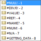
Inside the formula, we have the following code.
|
1 |
IF(ERROR.TYPE(DGET(C1:C5,1,A1:A2))=3 |
It means when the returned value is #VALUE!, then it shows “No student”. If the condition is not met then the error is #NUM! and the returned value must be “Duplicated student”.
Removing duplicates from a range
To delete duplicates, first select cells with data.
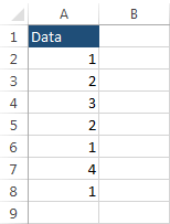
Then go to DATA >> Data Tools and click the Remove Duplicates button. A new window will appear.
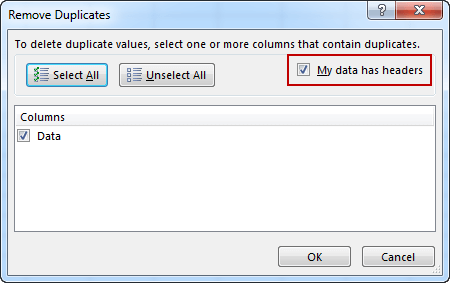
Because our data has a header, check My data has headers.
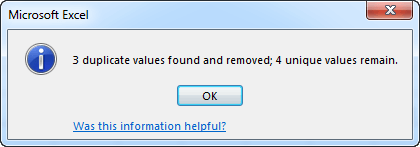
The new window appears. It shows the information on how many cells were removed and how many unique items remained.
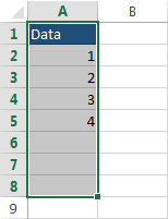
The result is as follows.
Removing duplicates from a table using Advanced Filter
Another trick to delete duplicates is by using the Advanced filter.
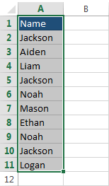
Example:
First, select the data where you want to remove duplicates.
Go to DATA >> Sort & Filter and click the Advanced button.
A new window will appear.
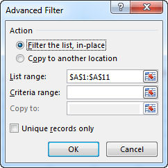
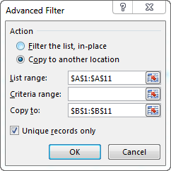
Now you need to copy data to another location. Let’s copy it to the next column. Choose Copy to another location and change $A$1:$A$12 to $B$1:$B$12. This will copy the cells to column B. What you also need to do is to check Unique records only.
And the result.
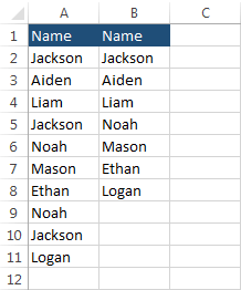
Only unique values were copied.
Removing duplicates based on several columns
Normally when you delete duplicates you analyze only a single column, but sometimes you need to take into consideration two or more.
The following example will illustrate you how you can remove duplicates based on several columns.
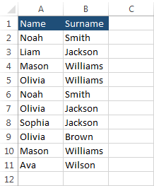
Select the data, then choose DATA >> Data Tools >> Remove Duplicates. If you check only Name you will get the following result.
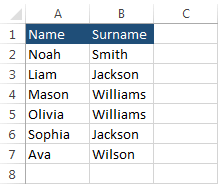
As you can see all names in the A table are unique. Now, do the same, but this time with the surnames and your result will be as follows.
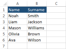
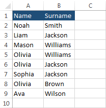
Just as with names, all values are unique. Now keep both tables checked. This time, Excel removed only two rows, the first with Noah Smith and the second with Mason Williams.
Removing duplicates automatically
In order to remove entered duplicates automatically, you need to do two things
- Record a macro to know how the code for removing duplicates looks like.
- Create an event.
Enter any value in cell A2. If you do it only for cell A1 Excel will display the following error.

NOTICE
If you enter a value to cell A2, then delete it and enter it to cell A1, or if you just move the value of cell A2 to A1, Excel won’t display the error.
Select cells A1:A10 and start recording a macro. After creating a name, click OK. Now, go to DATA >> Data Tools >> Remove Duplicates.
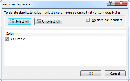
Column A should be selected. Click OK.
Stop the macro.
Go to VIEW >> Macros >> Macros.
Copy the following part of the macro and edit the range, changing it to A1:A10.
|
1 |
ActiveSheet.Range("$A$1:$A$10").RemoveDuplicates Columns:=1, Header:=xlNo |
CAUTION
Don’t use ActiveSheet.Range(“A”) because Excel will return an error.
In the second part, we need to create an event.
Open the VBA window (Alt + F11), double-click the current sheet, then choose worksheet and SelectionChange. This will execute the code each time you change something in the worksheet. Now, enter the previous code inside the Subroutine.
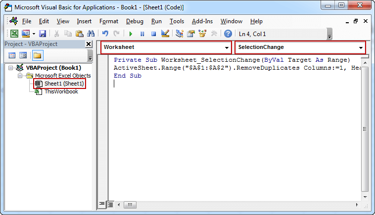
CAUTION
Choose Worksheet, instead of Workbook, otherwise, Excel will return an error.
Each time you enter the value that is duplicated, Excel will remove it automatically.
Finding duplicates using the Pivot table
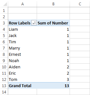
This time we will count the number of duplicates using a pivot table.
Example:
First, create the following table.
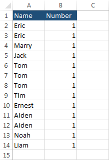
Click any cell inside the table and choose INSERT >> Tables >> PivotTable.
When a new window appears, click OK. Now check both Name and Number.
Sort your table and you will get the following result.
