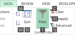
In this lesson, I will show you how you can use keyboard shortcuts to manipulate filters in Excel.
Create filters
Take a look at the following example.
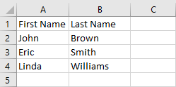
To create a filter with a keyboard shortcut, click a cell inside the data and use Ctrl + T or Ctrl + L shortcut. It will transform your data into a table. Excel will ask you whether your data has headers or not.
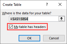
In this example, we have headers (First Name, Last Name) so you have to check this option.
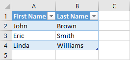
The new icons, called filter icons appeared to the right of the names of the headers.
Turn Filters On or Off
There is another way to create filter icons using keyboard shortcuts: Ctrl + Shift + L.
With these keys, you can, just like in the previous method, create filter icons. This time, you need to have headers in the columns.
Our example has headers, so we can use this method.
Click any cell inside the data and use the shortcut. It will add filter icons, the same way as when we were creating a table, but this time we won’t be asked whether our columns have headers, and it doesn’t format our cells visually.
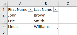
To turn off filter icons use Ctrl + Shift + L again.
CAUTION
When you use the Ctrl + Shift + L keyboard shortcut to turn off filtering, all your filtering options will be lost.
Access filter drop-down menu
You can access the filter drop-down menu with a keyboard shortcut. But first, you need to move your cursor to the column header. Now, you can use Left Alt + ↓ shortcut.
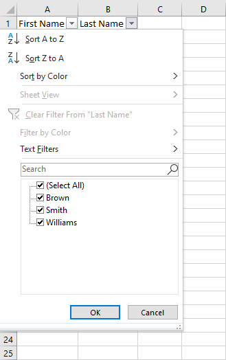
You can navigate through the menu options using the Tab key to go forward. Shift + Tab to go backward or use Arrow Keys.
To reveal additional options under a selection, use the Right Arrow key.
Check/Uncheck Filter Items
The unique filter items appear at the bottom of the filter menu.
If you want to select or unselect table elements, move to this element and use Spacebar.
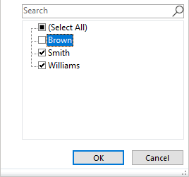
It will either select or deselect highlighted item. To confirm your filtering option press the Enter key.
Access Search Box
Since Excel 2010, the Search box was added as a new feature. It’s also present in Excel 365.
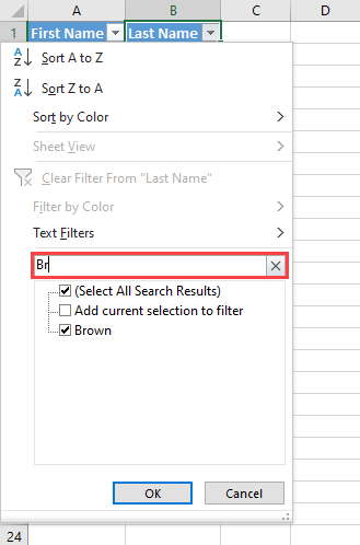
You can easily access it with your keyboard. First, click the name of a table header and then use Left Alt + Down Arrow to expand filtering options.
The last thing to do is to press the letter “e” on your keyboard.
That’s all, you can type a phrase, you want to use and Excel will filter the data based on your entry.
Drop-Down Menu Shortcuts
You don’t have to navigate through elements using arrows or tabs, but you can also use keyboard shortcuts. After you use the Left Alt + ↓ shortcut you can use one of the following.
S – Sort A to Z
O – Sort Z to A
T – Sort by color
C – Clear filter
I – Filter by color
F – Text filters
E – Text box
Clear All Filters in a Column
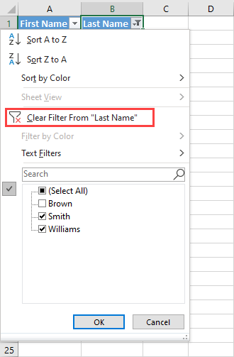
A quick and easy way to clear all filters in a particular column is to use a simple keyboard shortcut.
Press Left Alt + Down Arrow as you did before.
Now, when the filtering options are expanded, press “c”. This will remove all filters from the column.
Clear All Filters at Once
In the previous example, I showed you how you can clear the filter in one column. In this part, you will learn how you can clear filters in all columns using your keyboard.
This is not the standard keyboard shortcut because this time we will press one key after another.
Press Alt >> A >> C to clear all filters.
