Find Last Cell with Value in a Row in Excel

Finding the last cell with value in a row is a very common task in Excel. It can be very time-consuming especially if we are working with a very large dataset.

In this tutorial, we will look at the following 4 easy methods that we can use to find the last cell with value.

Use Ctrl + Right Arrow Key

Using the keyboard shortcut Ctrl + Right Arrow is the fastest way of finding the last non-blank cell in a Row that does not have gaps.

Select the first cell in the row and press Ctrl + Right Arrow. The cell selector will move to the last cell with a value in that row:

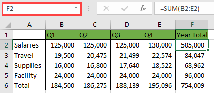
We can see the address of the last non-blank cell (F2) in row 2 in the Name Box.

This method takes us to the last non-blank cell in contiguous data.

Use Ctrl + Left Arrow Key

If the row has blank cells before the last cell with data, using Ctrl + Right Arrow will not take us to the last cell with a value:

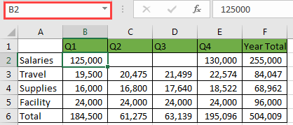
It will take us to Cell B2 which is the first cell with a value just before the first blank cell.

For us to get to the last cell with a value in this case, we use the following steps:

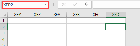
1. Type XFD2 in the Name Box and press Enter. The cell selector moves to cell XFD2 which is the very last cell in Row 2:

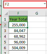
2. Press the keyboard shortcut Ctrl + Left Arrow. The cell selector will move back to cell F2 which is the last cell with a value in Row 2:

This method is the sure-fire way of finding the last cell with a value in a row in Excel.

Use ADDRESS and MATCH functions

The ADDRESS function creates a cell reference as text, given specified row and column numbers.

The MATCH function returns the relative position of an item in an array that matches a specified value in a specified order.

The syntax of the MATCH function is:

MATCH(lookup_value, lookup_array, [match_type])

The match_type argument is optional and it can be a 1,0, or -1. The 1 stands for Less than and finds the largest value that is less than or equal to the look_up value. The lookup_array must be in the ascending order.

The 0 stands for Exact match and finds the first value that is exactly equal to the lookup_value. The lookup_array can be in any order.

The -1 stands for Greater than and finds the smallest value that is greater than or equal to the lookup_value. The lookup_array must be in descending order.

We will use the following dataset to show how we can use the combination of ADRESS and MATCH functions to find the address of the last cell with value in a row in Excel:

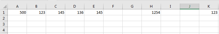
We use the following steps:

1. Select Cell A2 and type in the formula =ADDRESS(1,MATCH(2,1/(1:1<>””),1),4)
2. Press Ctrl + Shift + Enter to enter the formula since it is an array formula:

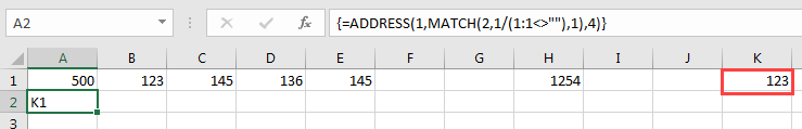
The formula returns K1 as the cell address for the last cell in Row 1 with value. This formula returns the address of the last non-empty cell in the row while ignoring blanks.

Explanation of the Formula

• 1:1<>”” – this part of the formula returns TRUE or 1 if a cell in Row 1 has a value and returns FALSE or 0 if it has no value.
• 1/(1:1<>”” – In this part, if there is a value in a cell, the formula becomes 1/1 and if the cell doesn’t have a value the formula becomes 1/0. This means that the output is either 1 or an error value of #DIV/0!
• MATCH(2,1/(1:1<>””),1) returns value 11. The MATCH function checked the values up to the last cell in the row and backed up passing all the zeroes and landed on the first value 1 in Column K which is column number 11. In this case, all the other numbers from the left are zeroes and the value 1 in column K is the first largest value that is less than or equal to the lookup value of 2.
• ADDRESS(1,MATCH(2,1/(1:1<>””),1),4) becomes ADDRESS(1,11,4). 1 stands for Row 1, 11 for column K, and 4 is for relative referencing. The formula returns the cell address K1.

Use Excel VBA

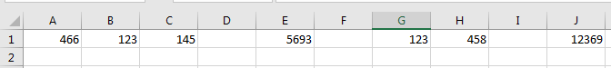
We will use the following dataset to show how we can use Excel VBA to find the last cell with value in a given row:

We use the following steps:

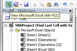
1. In the active worksheet press Alt + F11 to switch to the Visual Basic Editor.
2. In the Project Window right-click the workbook and insert a new module.
3. Type in the following code in the new module:

4. Save the macro and press Alt + F11 to switch back to the active worksheet. Alternatively, we can click on the View Microsoft Excel button on the toolbar:

5. In the active worksheet, ensure that the active cell is in the row we want to work with.
6. Press Alt + F8 to open the Macro dialog box:

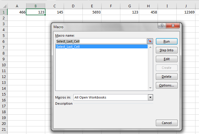
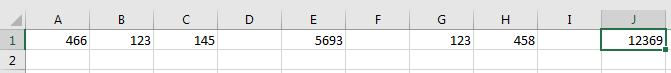
7. Click the Run button and the Cell Selector moves to Cell J1 which is the last cell with a value in Row 1:

Explanation of the Select_Last_Cell Macro

Sub Select_Last_Cell()

Dim i As Long

i = ActiveCell.Row

Cells(i, 16384).End(xlToLeft).Select

End Sub

• The variable i is declared with the Long data type.
• ActiveCell.Row returns the active cell’s row number and assigns it to the variable i.
• Cells(i, 16384).End(xlToLeft).Select moves to cell number 16384 in the active row which is the very last cell in the row. The End property allows us to move back in the left direction in the range using the xlToLeft constant. The last cell with a value in the row is found and selected.

Conclusion

Finding the last cell with value in a row is a common task in Excel but it can be very time-consuming especially if we are working with large datasets.

In this tutorial, we have looked at four methods that we can use to make this task less time-consuming. The methods are using the keyboard shortcut Ctrl + Right Arrow Key, using the shortcut Ctrl + Left Arrow Key, using the formula that combines ADRESS and MATCH functions, and using Excel VBA.

You can use the method that you are most comfortable with and that fits your situation.