Everybody that uses Excel will find Pivot Tables to be one of the most useful and most used tools. With it, we can observe our data in a lot more powerful way than we do with other tools.
In the example below, we will show how to find the maximum value in our Pivot Table, either related to specific fields or in general.
Find the Maximum Value in the Pivot Table
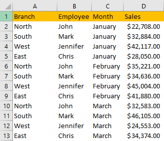
For our example, we will use the list of sales of different salespeople in imaginary branches:
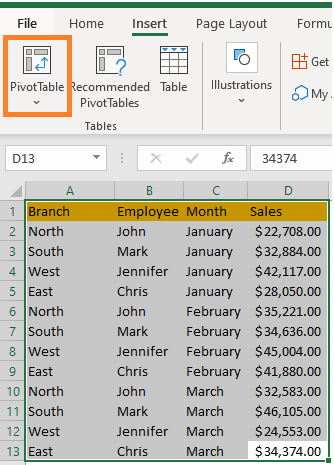
To create the Pivot Table, we will select our range, go to Insert >> Tables >> Pivot Table:
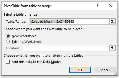
After that, we will simply click OK on the window that appears, and call this new sheet on which Pivot Table will be created “Pivot Table”:
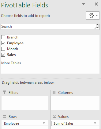
Once created, we will put Employee in Row Fields and Sales in Values field:
Our table looks like this:
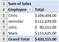
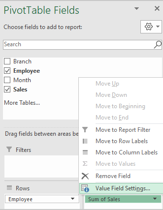
An automatic option that Excel presents for Values Field is, as you can see, Sum. So to change it to the maximum value, we can simply left-click on this field in Values and then select Value Field Settings:
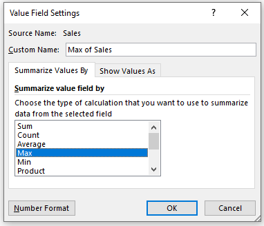
On the dialog that appears, we will choose the Max option and click OK:
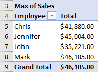
Once we do, our table will show only the maximum values for every Employee:
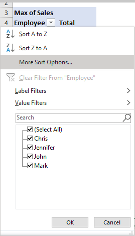
To find the max value of these four figures, we will click on the dropdown next to the Max of Sales Employee text, and then go to More Sort Options:
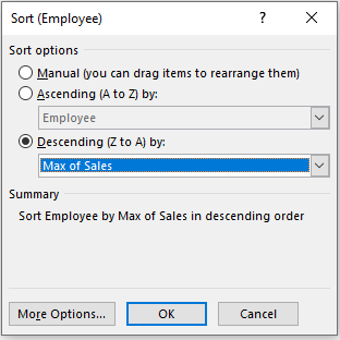
On the window that appears, we will choose Descending option and then choose Max of Sales as our option:
Our table looks like this now:
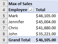
You will also notice that the number shown in Grand Total is identical to the maximum value. This is yet another, maybe easier way to check the maximum value in your Pivot Table.