Format Cell Based on a Different Cell in Excel

In Excel, there are limitless opportunities to format our data. One of the cool things that it is possible to do is to format certain cells on a basis of the values in different cells.

We can use any type of criteria to format any cell that we want.

Format Cells Based on the Cells in the same Sheet

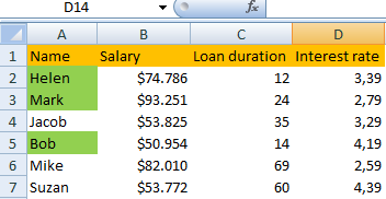
For our example, we will use the loans table with the name of the client, their annual salary, loan duration, and interest rate.

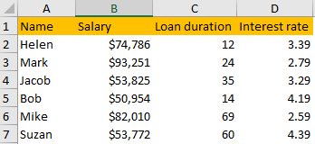
Now, we want to highlight the names of the client that have loan duration lower or equal to 24 months.

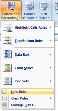
For this, we select range B2:B7 and go: to Home >> Styles >> Conditional Formatting >> New Rule:

In a pop-up window that appears, we will select Use a formula to determine which cells to format for a Rule Type, and then we will input our formula:

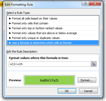
We have to determine the first cell in our range to be in the formula. This way, the format will be implemented to the same range in column B as well.

For the last part, we will define the format by clicking on Format…, going to the File tab, and selecting the color that we like (in our case, green color):

Once we click OK, we will notice that only the names of the clients that have loans with a duration lower or equal to 24 are affected:

Format Cells Based on the Cells in Different Sheet

In every Excel version since Office 2007 (this one is not included), it is possible to format the cells based on some condition that is determined in another sheet.

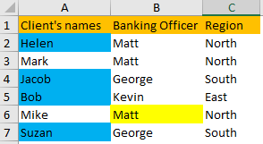
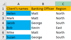
To show this, we have created another sheet in which clients’ names (same as in the first sheet), banking officers, and their working regions are presented:

We want to highlight all the clients that have an interest rate over 3.5. For this, we will select the range A2:A7, repeat our steps from the example above, and type in the formula

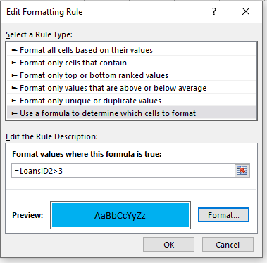
The only difference from the previous formula is that we are referencing another sheet. In this case, that sheet is the first one that we created and it is called “Loans”.

We will highlight the cells that match our criteria with blue color.

Our table now looks like this:

Since the use of condition is the usage of the IF function, it is possible to combine the conditions with AND or OR functions as well.

Let us suppose that we want to highlight only those banking officers who approved the loan for people with an annual salary over $70,000 and duration of the loan over 60 months.

Looking at our first table, we can see that we only have one such value and that the corresponding cell in the second sheet would be cell B6, meaning that Matt is the only one that satisfies the criteria.

We define this with the following formula:

We defined it in the edit formatting rule window, as usual:

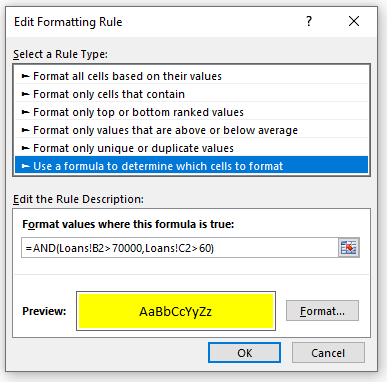
We can see that Matt is the only one highlighted, as already explained.