An Excel formula that uses cells from different worksheets has linked cells. You may need to go to linked cells in an Excel formula. This tutorial shows you how to go to linked cells in an Excel formula.
Example
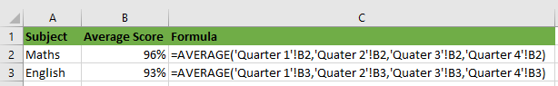
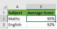
We will use the following dataset in our illustrations. The dataset has formulas that use four linked cells:
How to Go to Linked Cells in Excel Formula
We explain two methods that can be used to go to linked cells in an Excel formula.
Method 1: Use the Trace Precedents command on the Ribbon
We use the following steps:
- Select the cell that contains the formula. In this case, we select cell B2.
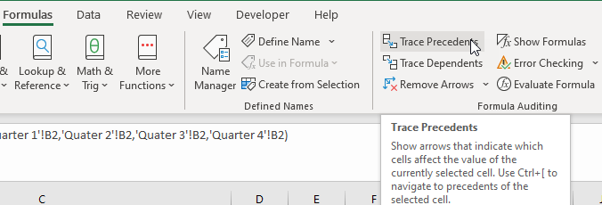
- Click Formulas >> Formula Auditing >> Trace Precedents.
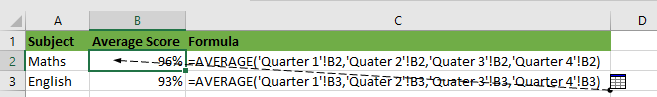
- Double-click the dotted line to open the Go To dialog box.
- All the linked cell references are displayed in the Go To list box. Select the first cell reference and click the OK button.
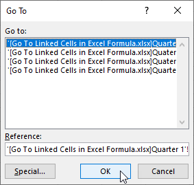
You are taken to the linked cell B2 that is in the Quarter 1 worksheet:
- Repeat steps 3 and 4 to go to the other linked cells.
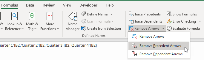
- Click Formulas >> Formula Auditing >> Remove Precedent Arrows to remove the arrow from the worksheet:
Method 2: Use the keyboard shortcut
- Select the cell that contains the formula. In this case, we select cell B3.
- Press Ctrl + [
You are taken to the first linked cell which is cell B3 in the Quarter 1 worksheet:

The limitation of this method is that it only takes you to the first linked cell in the formula. This is regardless of how many linked cells you have in your formula.
Conclusion
This tutorial explained two methods that can be used to go to linked cells in an Excel formula. We can use the Trace Precedents command or the Ctrl + [ keyboard shortcut.