Sometimes you have to switch columns with rows inside your table. This process is called transposing, and you can do it in Excel using a few different ways.
Let’s take a look at the following example:
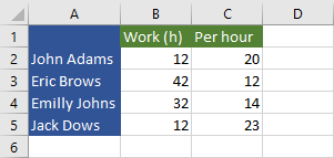
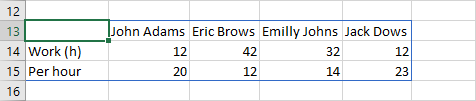
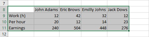
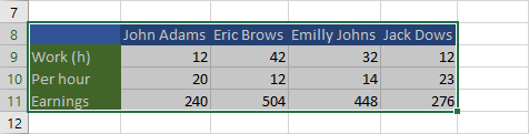
There are names of four people in the first column, the number of hours they worked in the second, and how much they earn per hour in the third one.
What we want to do here, is to switch columns with rows.
How to quickly transpose data
Follow these steps to transpose data:
- Select cells to copy.
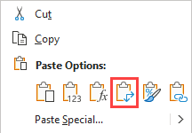
- Copy them (Ctrl + C).
- Choose a cell for the transposed table.
- Right-click and choose Transpose.
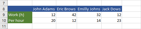
Columns and rows are switched after this operation. The formatting is preserved.
This is the quickest way to transpose data, but not the only one.
The TRANSPOSE function
When you copy data and paste it as transposed, the pasted data is not dynamic. This means that it doesn’t change automatically when you change the source.
This can be fixed with the TRANSPOSE function. Here’s how it works:
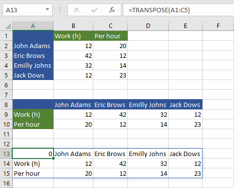
The function takes an array as a parameter and switches columns with rows. It doesn’t keep formatting, so if you want to have it, you need to apply it manually or use Format Painter.
Remove zero from the transpose
The problem with the previous example is that it shows 0 in a cell where the function is placed. You can quickly fix it using the following formula:
|
1 |
=TRANSPOSE(IF(A1:C5="","",A1:C5)) |
The formula inside the TRANSPOSE function copies the table from the source and if there is black space, it returns blank instead of 0.
Transpose with formatting and formulas
By default, when you use transpose by copy and paste, the formatting and formulas are preserved.
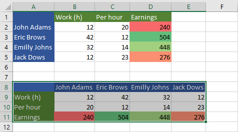
Let’s modify our example, to see how it works. Create an additional column with calculated earnings and transpose it by copying it the same way as before.
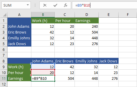
As you can see the formulas are preserved and reference the transposed cells correctly.
Transpose with formatting and values
If you want to automatically convert formulas to values, you have to use a different method.
First, copy the table as before, and then, instead o pasting it as transposed, click the Paste Special button.
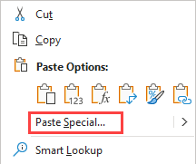
A new window will open. First, you have to check the Transpose option.
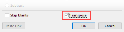
Let’s say that you want to convert all formulas to values, but also keep the formatting.
Because these are radio buttons, you have to choose one of them. There is no such option as Values and Formats, so you have to first copy one and then the other.
First, choose Values, check Transpose and click OK.
Next, repeat the same process, but this time instead of Values, choose Formats.
Transpose with condition
If you use conditional formatting in your example, and you try to paste values, the formatting won’t appear. If you try to paste only formatting, all formatting will be present without conditional formatting.
What you need to do is to paste both (one after another, the order is not important) Values and Formats.
Transpose with a keyboard shortcut
When you were pasting values as transposed, you may have noticed a letter (T) next to the button. This button allows you to quickly paste value without the need of navigating with your arrow keys.
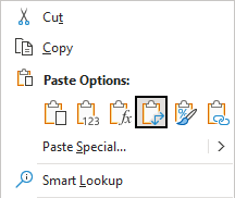
This quick shortcut is useful when you use Excel with your keyboard, instead of a mouse.
Use a macro keyboard shortcut
When you work with Excel with a keyboard, you can use Ctrl + V to paste values, but there is no shortcut to paste transposed values. This doesn’t mean you can’t do it. You can, with the help of the VBA code.
This doesn’t mean, you have to be a VBA programmer, just record a simple macro and see what the code looks like.
We are going to create a macro to paste transposed data and apply it to Ctrl + Shift + V.
First, copy the data and click the cell where you want to place it as transposed.
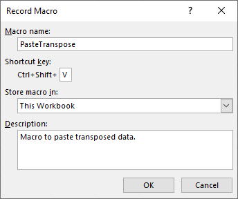
Next, navigate to View >> Macros and click Record Macro.

Inside the new window, name your macro and add a description, but what’s more important assign a keyboard shortcut.
We want to use Ctrl + Shift + V, so click inside the box next to Shortcut Key and press Shift + V. In macros Ctrl is added by default.
After you click the OK button, the macro starts recording. Inside the already selected cell paste transposed data and stop recording the macro.
Choose Ctrl + F11 to open the VBA code editor.
This is what the code looks like:
|
1 2 3 4 5 6 7 8 9 10 |
Sub PasteTranspose() ' ' PasteTranspose Macro ' Macro to paste transposed data. ' ' Keyboard Shortcut: Ctrl+Shift+V ' Selection.PasteSpecial Paste:=xlPasteAll, Operation:=xlNone, SkipBlanks:= _ False, Transpose:=True End Sub |
Besides the comment block, there are two lines of code. What is interesting is the following part:
|
1 |
Transpose:=True |
It indicates that the pasted data will be transposed.
Now, if you copy data, you can use the shortcut to paste it as transposed data.