We have seen how useful Slicers in Excel can be. They can help us filter our data set, and are especially good in combination with Pivot Tables and Pivot Charts.
One of the things that can be very frustrating when working with Slicers is that they can be easily moved and resized. Perhaps we do not want that to occur.
In the text below, we will show how exactly can we lock the position of Slicers, lock the cells in the sheet where Slicer is located, or lock the Slicer itself.
Lock the Position of a Slicer in Excel
As in the previous examples, we will use the list of NBA players, their teams, conferences, and statistics from several matches.
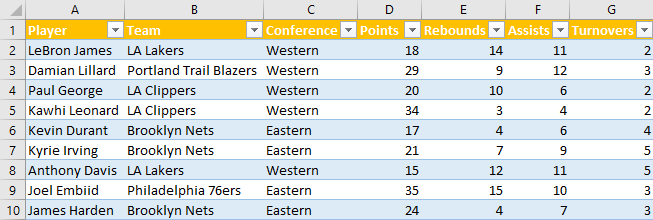
Our data set has 28 rows, but only 10 are presented in the table above.
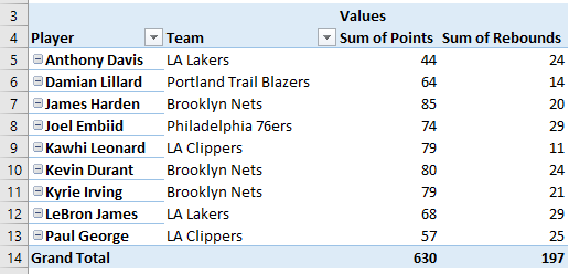
We will create the Pivot Table, put Players and Teams in the Rows field, and sum points and rebounds in the Values field.
Our table looks like this:
Next thing, we are going to create a Slicer by clicking on our Pivot Table, then going to PivotTable Tools >> Analyze >> Insert Slicer.
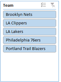
In a pop-up window that appears, we will select Teams and we have our Slicer:
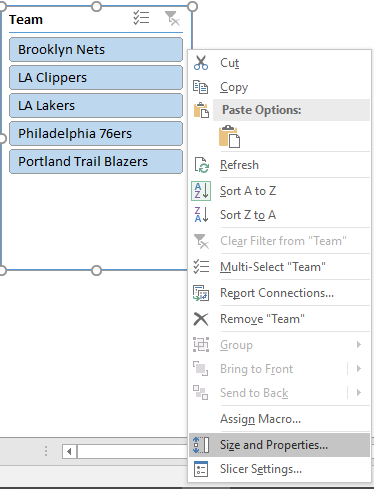
Currently created Slicer can be easily moved or resized in the sheet. To change this and to lock our Slicer in a certain way, we will right-click on it and then select Size and Properties.
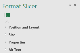
We will now have Format Slicer on the right side, with four options: Position and Layout, Size, Properties, and Alt Text to expand:
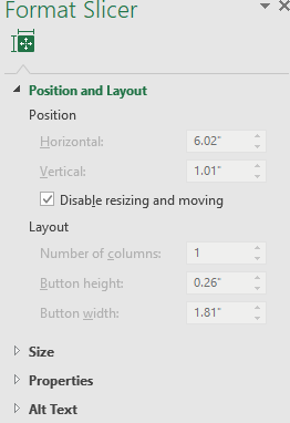
First, we have to expand the Position and Layout option. Then, we will click on Disable resizing and moving.
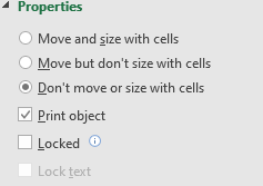
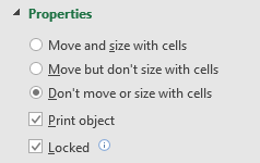
We now have to expand the Properties option. We will select the Don’t move or size with cells option and we will deselect Locked.
Now, our Slicer cannot be moved or resized.
Lock the Sheet and Allow Filtering
There is an option to lock the sheet but allow the filtering in our sheet. It is the same option as the one for locking the cells in Excel in general, with a couple of changes that have to be made.
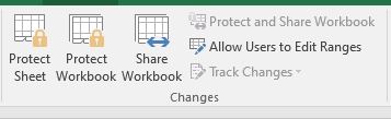
To lock the cells in our range, we will select it and then go to Review >> Changes >> Protect Sheet.
A pop-up window will appear. It looks like this:
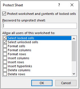
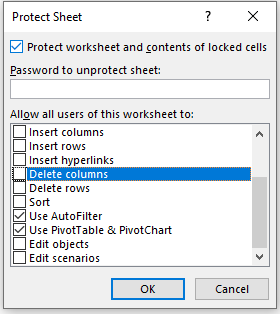
Select locked cells and Select unlocked cells fields will be checked by default. If not, we have to click on it. We have to scroll down to the end of the list and select Use AutoFilter and Use PivotTable & PivotChart as well:
When we finish this up, we can create our password to unprotect our sheet. We will put a simple password: „slicer“.
Excel will ask us to confirm this password one more time, with the warning message and information that the passwords are case-sensitive:
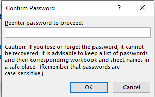
We will re-enter our password and click OK:
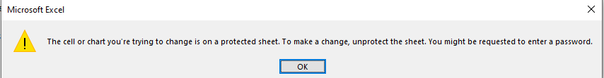
Now all of the cells in our sheet are locked, and we will get the following message if we want to make a change:
However, if we want to make changes to filters in our Slicer, we can still do that. For example, we will choose only the players from two teams- Brooklyn Nets and Portland Trail Blazers:
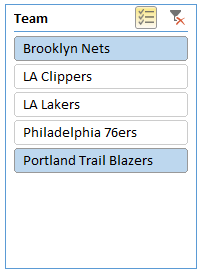
As seen, this will be allowed for us now, and these changes will be implemented in the Pivot Table as well.
Lock the Slicer
To lock the Slicer itself, we have to use the combination of the steps above. We will first unprotect our sheet (since we protected it before) by going to Review >> Changes >> Unprotect Sheets and inputting our password, then right-click on the Slicer, select Size and Properties, and check the Locked button in Properties:
Now, we will go to Protect Sheet option again and choose the same options as we did above.
Our password will be the same- slicer, and when we click OK, we now have our Slicer entirely locked and will not be able to select it or manipulate it in any way.