Use Name Manager in Excel

Most people use basic formulas in Excel, not wanting to „complicate“ things. Little that they know, these things are here for a reason, and the reason is to help you in your life.

One of these things is the name manager.

Definition of Excel Name Manager

Excel Name Manager is used to create, edit, delete and find names in the Excel workbook (or Excel sheet, depending on what you decide).

Excel Name Manager can be found in the Formulas tab.

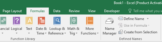
The Formulas tab is the default tab that is the one that can be found in the Excel ribbon by default. If you want to manage it, or you cannot find this tab or anything that you need (in this case Name Manager) just go anywhere on the gray area of the ribbon and choose the option Customize the Ribbon.

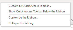
At this location, you can manage your ribbon and add all the Excel functions that you often use.

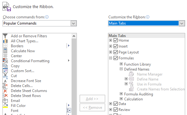
In the picture below, you can see that we have the option to choose from the tabs: All tabs, Main tabs, or Tool tabs.

To find the Formulas tab, we can choose the Main tabs. As seen, our Name Manager is under the subtab called Defined Names.

We can also access the Name Manager with the keyboard. To do this, we use the combination: Ctrl + F3. Name Manager is usually used to work with existing names. However, it also allows you to create a new name too. We will do just that in the following examples.

How to Define Ranges with Name Manager

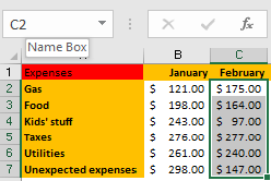
Let’s say that we have the table with expenses and revenues for a typical household for a time of one year, shown in months. The table could look like this:

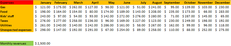
We have several categories of expenses: gas, food, kid’s stuff, taxes, utilities, and unexpected expenses.

For revenues, we have a fixed monthly value of $2.500.

If we select all the expenses for one month, let’s say January (not including the name of the month itself), and then click on our Name Manager in the Formulas tab, in the way described above, we should get a similar picture to the one below:

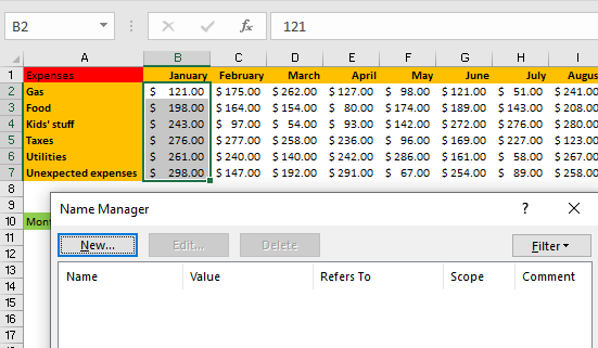
We will instantly get a pop-up window. Usually, this window will be in the middle. We dragged it to the left side to present it better in this case.

You can notice that the Name Manager has several columns to be populated: Name, Value, Refers to, Scope and Comment.

If you now click on the button New we can find out how these should be used in an example.

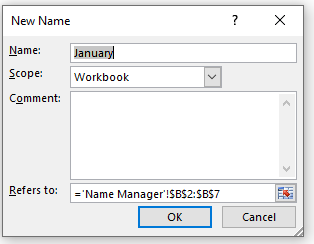
Name: Excel is smart enough to recognize that we took all the data in the column beneath the word January so it automatically gives the name January to our range. This is only a suggestion from Excel as we can choose any name that we find suitable.

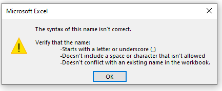
Now, there are some limits to this as we are not allowed to name our range the following:

• It cannot start with a letter or underscore (_)
• Cannot include a space, or character that is not allowed
• Cannot conflict with an existing name in the workbook

If you try any of these things, a pop-up will appear with the above-stated instructions:

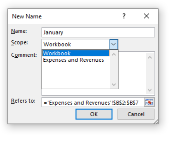
Scope: Here we determine whether a named range is local to a given worksheet or global across the entire workbook. Global names have a scope of a workbook, and local names have a scope equal to the sheet name they exist on.

In our example, we can choose between the sheet (we named our sheet Expenses and Revenues) and the Workbook. I will choose the workbook, in case I need this named range in other sheets as well.

Comment– In this section, we can write anything, possibly explaining our range or the reason behind the name of our range.

Refers to: This is the part where we choose the cells on which our Name Manager applies. We already selected our January expenses for this purpose (cells B2:B7). You will notice that the Refer to functions as a formula and that it „hard-codes“ the range that you select (picture above).

When we say „hard-code“ we mean the dollar symbol that we already explained in previous articles.

When we finish up our range, we simply click the OK button.

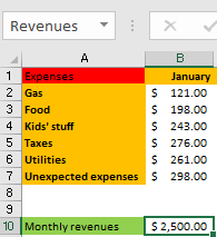
There is also an easier way to define a range with the Name Manager. We will do this in February. When we select all the expenses for February, we can see this name box in the top left corner (picture below).

Currently, our name refers to the first cell that we initially selected. We can simply change the name of our selected range to February.

To find your named ranges, you simply go to Name Manager in the Formulas tab (explained above) and click on the icon. We will see our January and February ranges defined.

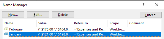
We have some options for managing our named ranges: New (creates new name range), Edit (changes the scope), or Delete (deletes some of the name ranges).

The final option is Filter, which allows us to filter our name ranges in various ways:

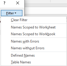
• Names Scoped to Worksheet or Names Scroped to Workbook– This filters out our Scope of the named ranges.
• Names with Errors or Names without Errors.
• Defined Names– If we defined a name for some range (we did in our case).
• Table Names– If our range is a table.

The Use of Name Manager

For further purposes, we will define all months of the year with the name manager. We also created a name for our yearly expenses and named it Yearly_expenses. Finally, we defined cell B10 (our revenue) and name it simply: Revenues

The best thing about Name Manager is that all the things that we defined above can be used in our formulas. That is the reason why the Name Manager is located in the Formulas tab in the first place.

We will open up another worksheet and call it Calculations. Remember, if we have chosen the worksheet for a scope of the name range before, it could not be used in another worksheet.

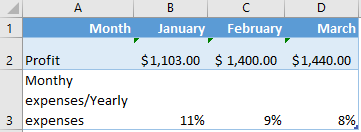
Our table in sheet Calculation has three rows: Month, Profit, and Monthy expenses/Yearly expenses. To simplify, we are calculating the data for the first three months only.

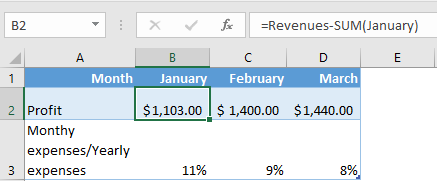
Now, the profit row should calculate the difference between the revenues and the expenses for the given month. Since we have it all defined, the function in our B2 cell is as follows:

As seen, we do not have to use ranges to define our formula, as we already did. When creating the formula, you just need to type the word you named your range.

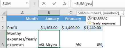
For example, if we want to find out the percentage of January expenses in total yearly expenses, we first have to find the sum of yearly expenses. We have a named range for these expenses, so we type in:

As soon as we give out our info regarding the name range that we want to use, a suggestion for us in a so-called IntelliSense will appear. IntelliSense determines which variable or function the user most likely needs (picture above)

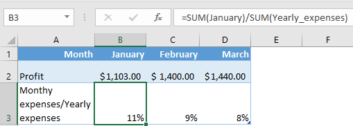
The same thing will be suggested when we start to type in January, so our formula in B3 will be:

For all of the other months, we just need to change the name range in our formulas. Since we already have the ranges defined, it should not take us much time.

There are easier ways to perform calculations that were used in this example. This was just to show the use of Name Manager. It can get pretty handy when we want to manipulate a certain range in many ways and many worksheets, and we want to „call it“ in a function without much trouble.