Random Question Generator in Excel

We can use Excel for many purposes that would not come to your mind when we first tackle a certain issue.

In the example below, we will show how to make a random question generator in Excel. We will only use formulas (multiple ones) to achieve this.

Creating Questions

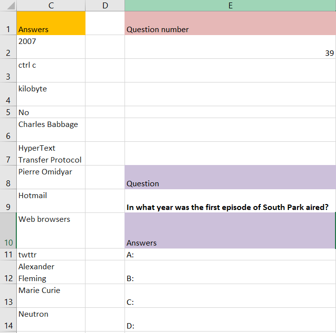
The first thing that we need to do is to create questions. We have created a list of 51 various questions. They look like this:

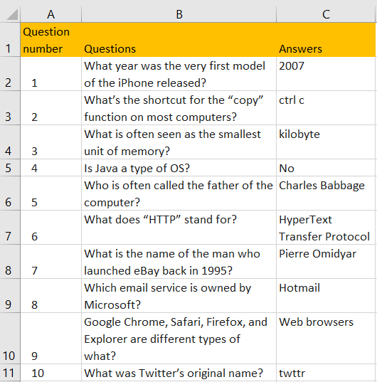
Some of these questions are related, and some are not, so do not be confused if you stumble upon some illogical answers down the road.

The first thing we need to do is to find a way in which we can generate random questions from our list. We will do this by using the RANDBETWEEN function. This function only searches for two parameters, lower bound and upper bound. We will input numbers 1 and 46. This is our formula:

And we will insert it into b:

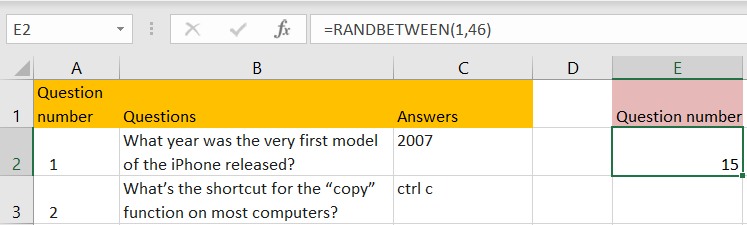
Although we have 51 total questions, we will go to the number 46, because we will prepare the series of right and wrong answers, and wrong answers will be equal to the right answer plus a number down the list in the answers column, and we do not want to get stuck with null as an answer.

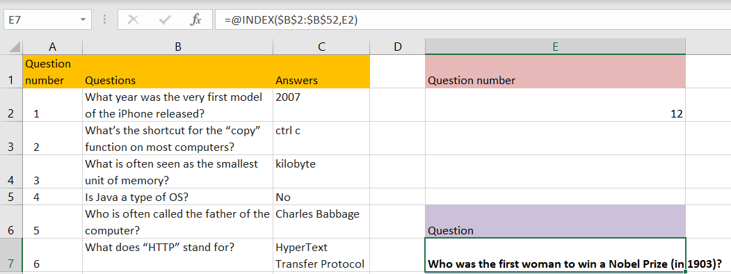
For the next thing, we will derive the actual question from the question number. We will use the INDEX formula for this purpose. We will insert the formula in cell E7:

Since RANDBETWEEN changes every time when we perform an action in Excel, we will generate a new question every time. This is what the question looks like in the worksheet:

Creating Answers

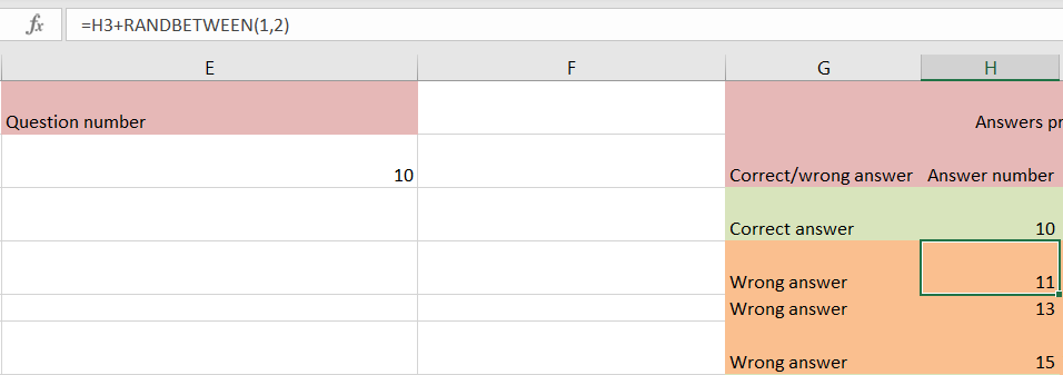
On the right side, we will do the preparation of the answers. We will insert four possible answers into four rows. The first row will be reserved for the right answer, and the rest of them will be for the wrong ones. Next to these, in the adjacent column, we will put in the question number, and then we will put in that number plus one or two, which will give us the answers down our list:

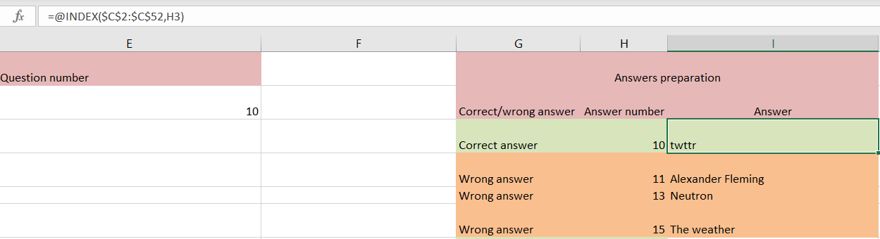
In column I, we will use the INDEX formula to find the answers to questions based on the number in column H. This is the formula that we will use:

Our array will be all the answers in column C, and our row number will be located in column H. We will insert the formula in cell I3, and then drag it to the cell I6:

Now, we have a question generator, and we have the answers all set as well. But, as it can be seen, even if we do not mark correct and wrong answers, the users could still figure out that the right answers are located in the first place.

Randomizing Answers

We need to make this order random as well. To do this, we will add two columns, and in the first one next to our table, we will use the RAND function (this function randomly gives out a number between 0 and 1). The formula that we will input in cell G3 will be:

We will drag this formula to the end of a table:

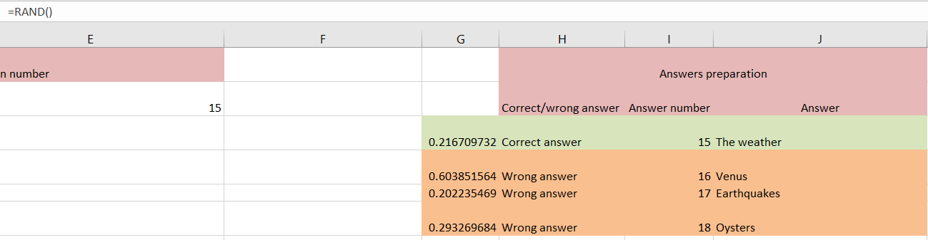
Every time we perform an action in our sheet, these numbers will change. Since they will always be different, this means that sometimes the right answer will have the largest number, and sometimes one of the wrong ones will.

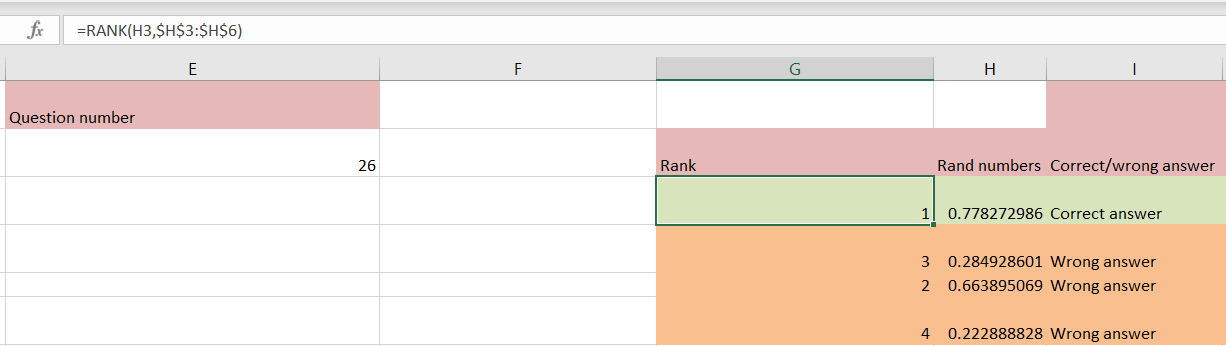
Now we need to rank these numbers, from largest to smallest. To do this, we will use the RANK function. The RANK function uses two parameters: number and reference. This will be the function we will use in cell G3 (we will add another column prior):

We will drag the formula till the end of our table, and this will be our result:

At this point, we have a question number randomized, and we have the proposed answers as well (one correct answer and three wrong ones).

Listing the Answers

What we need now is to list the answers to our questions. We will do that in column E:

Now we need to add the potential answers in the adjacent column. In the same row in which we have answer “A:” we will insert the following formula in column F (that will be cell F11):

To explain this formula: We use the ROW formula to reference our lookup_value, and we are searching for answers. Our table array is our newly created table for answer preparation, and the column index number is number 5, which means we will derive the answers that we have in this table:

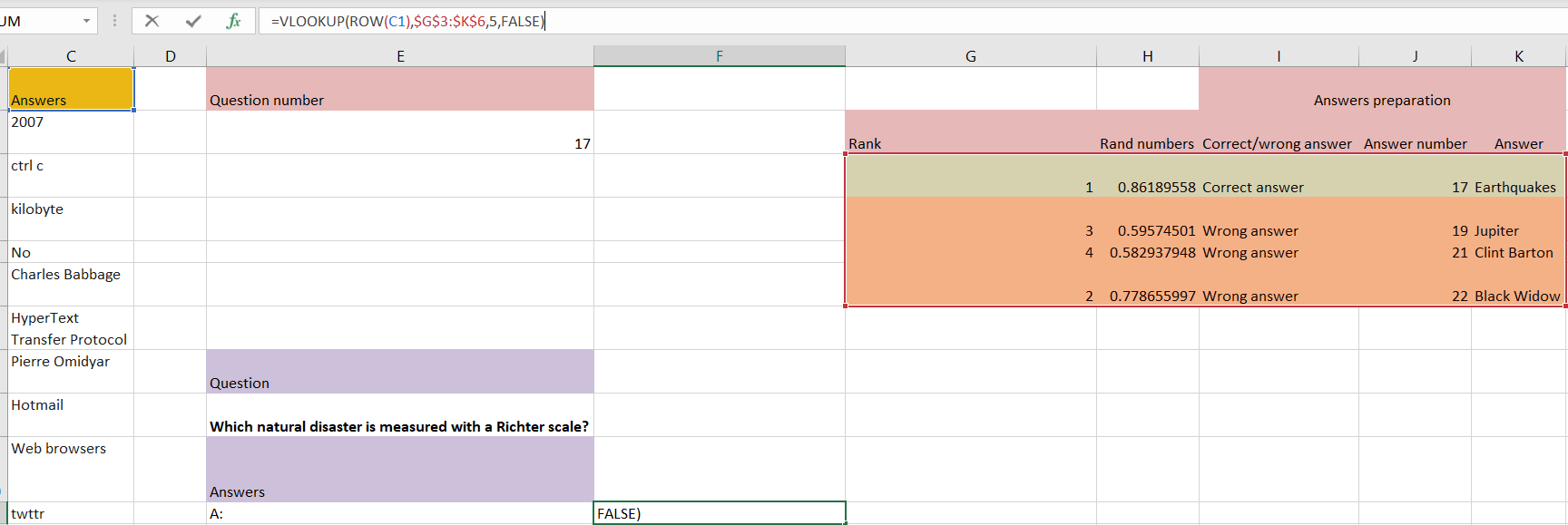
Using ROW in our formula will allow us to show the answers based on their rank, meaning that the right answers will be shuffled.

Our final product looks like this:

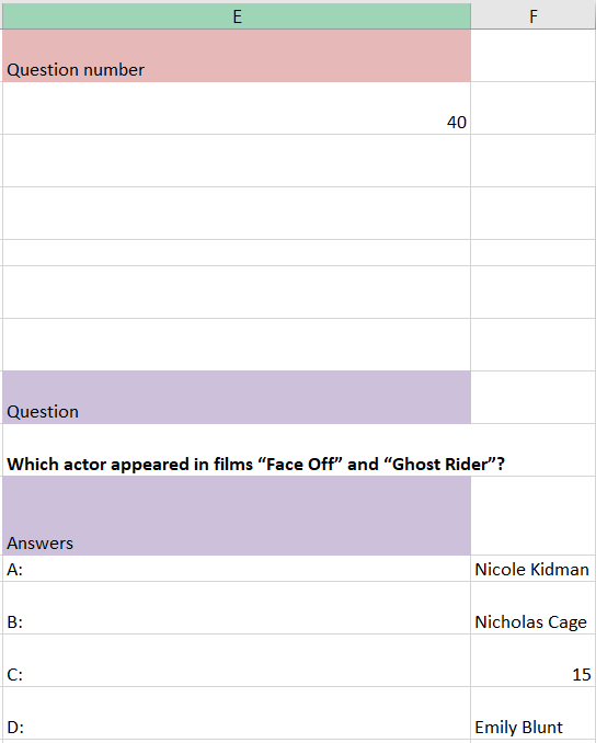
As said in the beginning, the questions and answers from our pool do not make much sense, but you can always create your own list of questions and answers, and also use RANDBETWEEN to manipulate the scope of possible wrong answers.