Using Pivot Tables in Excel, and Slicers alongside them is a great way of filtering data sets and extracting desired results from them. There are multiple options and neat tricks that can be used to make the data more visually presentable.
In the example below, we will show how to remove possible blanks from the slicer.
Remove Blanks from Slicers
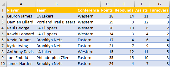
For the example, we will use the list of NBA players from different teams and conferences, and their statistics from several categories (points, rebounds, assists, and turnovers):
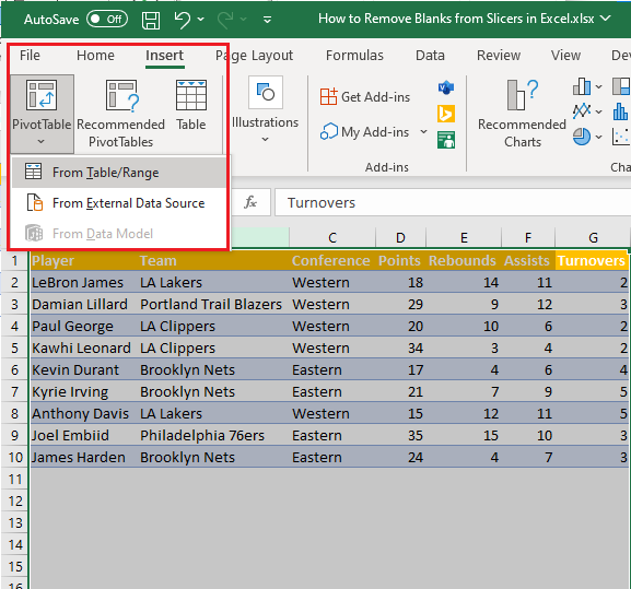
We will create a pivot table now, by selecting all columns where our data is located, so columns A:G, and then go to Insert >> Tables >> PivotTable >> From Table/Range:
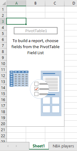
On a pop-up window, we will simply click OK, and a Pivot Table will be inserted into the new sheet:
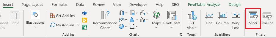
We will click on the Pivot Table, and then go to Insert >> Filters >> Slicer:
Once we click on it, we will have a Slicer window opened:
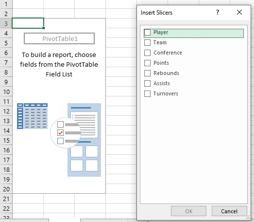
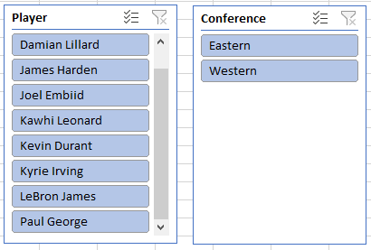
We can choose any Slider that we want- in our case, that will be Player and Conference:
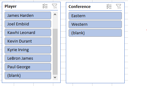
It is noticeable that we have blanks at the end of our slicers. The reason for this is that we included all the data from columns, not only the range where our data is located. We have two solutions to this issue:
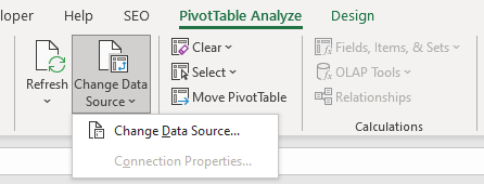
We can click on the Pivot Table and then go to PivotTable Analyze >> Data >> Change Data Source:
After that, we will select only the range where our data is located, which is range A1:G10:
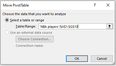
When we click OK, we will not have blanks in our Slicers:
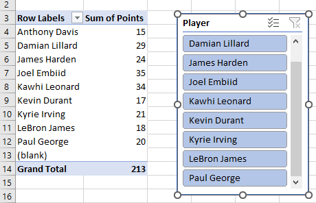
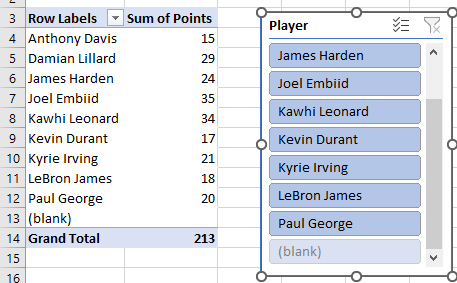
We can insert the data in the Pivot table, for example, Player in Rows, and Points in Values, and then we will see that the word Blank is shaded:
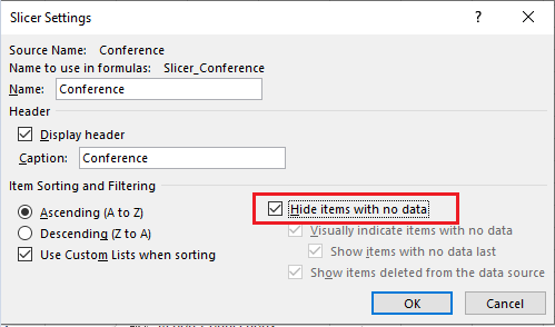
We will then right-click on the Slicer, and choose Slicer Settings:
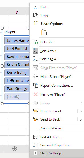
Once on the Slicer Settings window, we will check the box Hide items with no data:
And we will have the Blanks removed from Slicer, although the blanks will still be present in the Pivot Table: