When we talk about Pivot Tables in Excel, we usually discuss all of the good things that they bring to our lives.
So far, however, little has been said about manipulating the looks of the Pivot Table and the problems that we can encounter in creating one.
We will try to present and answer one of those problems in the text below and that is: how to remove duplicates from the Pivot Table?
Remove Duplicates by Removing Subtotals
For our example, let us say that we have a table with various colors and seasons (Spring, Summer, Autumn, and Winter). This table is completely random and has no meaning:
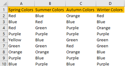
Now, we will select our range and create Pivot Table by going to Insert >> Tables >> Pivot Tables and inserting the table into the new sheet that we are simply going to call “Pivot Table”.
We will select only Spring and Summer colors to be in our Rows fields.
Our Pivot Table looks like this:

Pivot Table should be useful in gathering all the data together and removing duplicates. The table that we have created does not do that. We have a lot of duplicates in the same column. So we are going to make a few adjustments.
First, we will right-click anywhere on the table and select PivotTable Options:

In the pop-up window that appears, we will go to Display and then select Classic PivotTable layout (enables dragging of fields in the grid)
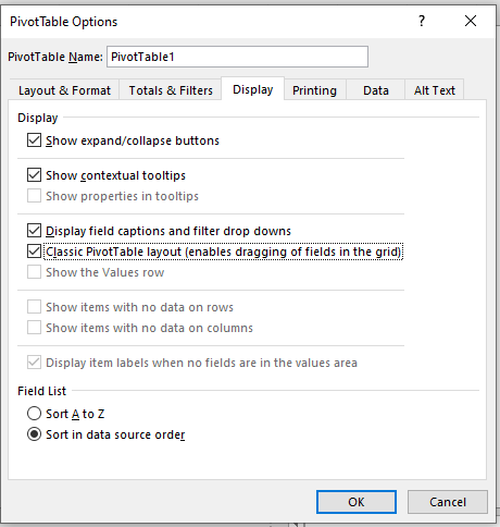
Our table now looks like this:
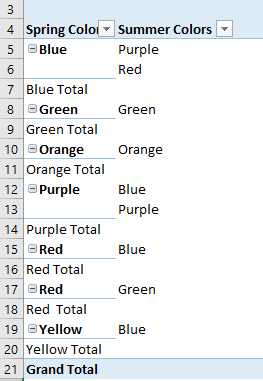
It is noticeable that we now have these boring totals shown: Blue Total, Green Total, and so on.
To remove those, we will right-click in the column with Spring Colors data and unselect Subtotal “Sprint Colors”:
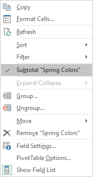
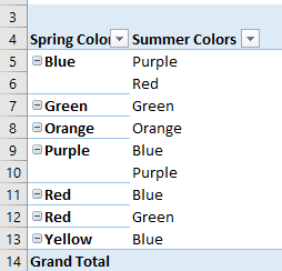
When we do this, our table will be much neater, and will finally look like this:
Remove Duplicates by Making Sure Source Data is the Same
Although it can seem like a rookie mistake, sometimes we can have typos in our data. If you watched carefully, you could notice that we have our “Red” color appearing twice in the table from the first example. Why is that the case?
When we go to our data source table, we can see that the Red color is in the second and fourth rows. In the second row, this color is written only as “Red”, while in the fourth row, it is written as “Red “, with the blank space after the word itself.
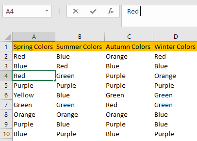
Because of this, our Pivot Table is showing two Red colors in column A.
When we remove the blank sign and go to our Pivot Table, select it, and go to PivotTable Tools >> Analyze >> Refresh, our data will now change:
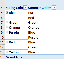
Now we only have one “Red” color in our Spring Color column.
Remove Duplicates with Data Formatting
There could be one more reason why the Pivot Table is showing duplicates. We will create a column with random numbers that are ranging from 1 to 20 and will call it simply „Numbers“. We will change the sheet name to „Colors and Numbers“ as well.

In our example, it is painfully obvious that two numbers: 4 and 16 are differently formatted in comparison with other numbers in the list.
In this case, these two cells are formatted as Text, while all the other numbers are formatted as General. This is only a micro example. If you had a large data set, this could not be so easy to notice.
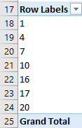
If we would go on to create a Pivot Table to find unique values, you will have numbers 4 and 16 appearing two times:
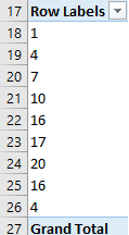
To make sure that the data set is formatted in the same way, we cannot simply select our column and change the formatting. This will not do the trick. Furthermore, it would be time-consuming to find all of the cells with different formatting.
To resolve this issue, we will select the numbers column, go to Data >> Data Tools >> Text to Columns:

Once we click on it, a pop-up will appear, showing us the Convert Text to Columns Wizard, which has three steps:
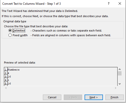
For the first step, we will choose delimited as the file type that best describes our data and clicks Next
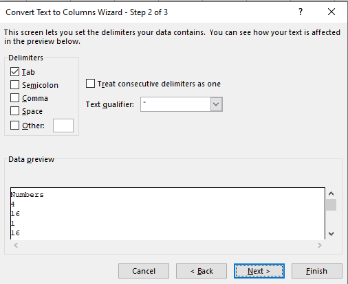
In the second step, we can choose Tab or not choose any delimiter at all. Our goal here is not to separate the text in cells (which delimiters usually do), but to format the data so that it is consistent.
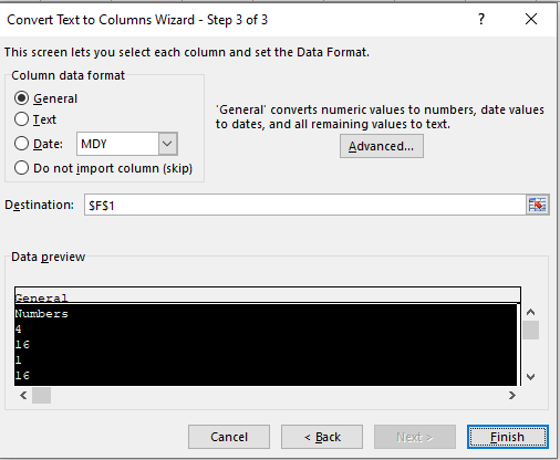
For the final step, we will select General and click Finish.
Our Number column now looks fine:

For the final step, we have to go to the Pivot Table we created, click on it, then go to Analyze in Pivot Table Tools and click on Refresh (as we did before):

When we do that, our Pivot Table will show unique values, as it should.
