Remove Table Formatting in Excel

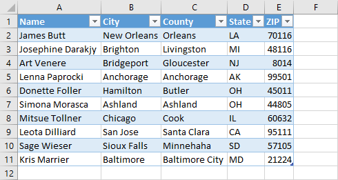
If you create a table from data, Excel will automatically apply a default formatting to it.

Let’s see how it works in practice.

We have a list of people’s names, cities, etc.

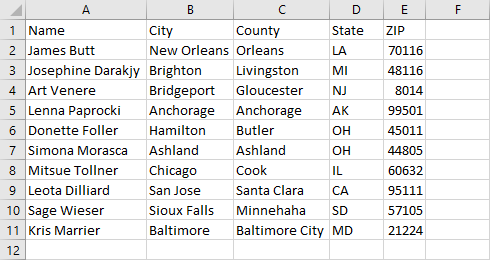
If you click any cell inside this data and create a table (Ctrl + T), Excel will create a table with the default formatting.

Clear Formatting using the Home Tab

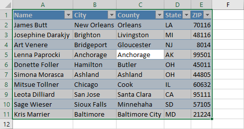
Select all cells in the table. You can do it by clicking a header cell and pressing Ctrl + A. You can also click any cell inside a table (but header cells) and press Ctrl + A twice. If you press the shortcut once, Excel won’t select header cells.

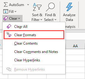
 Navigate to Home >> Editing >> Clear and click Clear Format.

All that, the table formatting is gone but the functionality of the table is still there.

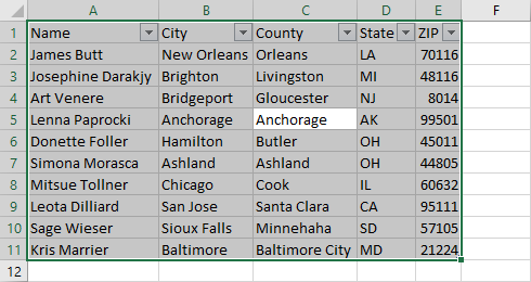
You can’t clear formatting for the part of a table. If you don’t select all the cells and click Clear Formats, nothing changes, the formatting will stay as it was before.

Clear Formatting using the Table Design Tab

Another, yet similar way to remove formatting from the table is to use the Table Design Tab. This is the special tab that appears when you click a cell inside a table.

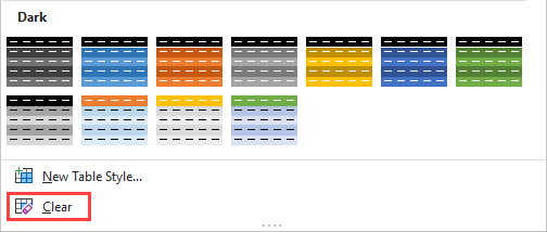
Click this tab, and then under Table Styles, select the More button.

If you move to the very bottom of the expanded window, there is the Clear button.

Click it to remove the formatting. The difference between this method and the last one is that, here, you don’t have to select all the cells. Excel knows that this is a table and you want to apply this to all these cells.

Clear Formatting by Selecting a Different Style

If you navigate to Table Styles and click the More button, you’ll notice that one formatting is different than the others.

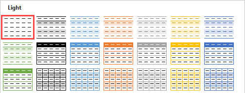
Hover a mouse cursor over it. It says None. If you click it, it will act the same as the Clear button from the previous step.

Convert Table to Range

It’s very easy to convert Excel data to a table, but it’s also easy to revert the process and convert a table back to the range.

To do it, click the table and go to Table Design >> Tools >> Convert to Range.

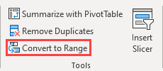
After you click the button, you’ll notice that the filtering buttons disappeared from the table headers.  This means that the table was successfully converted to the range.

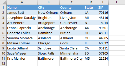
Remove Formatting from the Part of the Range

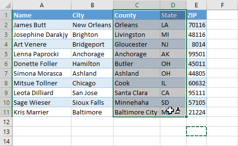
You can’t remove formatting from the part of the table using the Clear Formats button, but you can do it if you convert it to the range.

Select cells from C1 to D11 and navigate to Home >> Editing >> Clear >> Clear Formats.

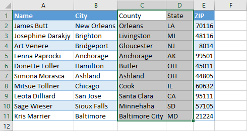
If you convert this range to a table, it will format the whole table again.

Remove Formatting using the Format Painter

Excel offers a feature called Format Painter. It applies formatting from the selected cell to the cells that you choose.

To replicate the last example using this tool, first, select a cell outside the range, where no formatting is applied (for example, E13), and navigate to Home >> Clipboard and choose Format Painter.

Now, drag cells from C1 to D11 to apply new formatting. Because you selected a cell with no formatting, the new format is like removing all formatting from cells.

Create a Macro and Apply Shortcut

You can remove formatting using the VBA code. If you are not an expert in VBA, don’t worry a macro recorder will help you with that.

Click a cell inside the table. In the bottom-left part of the screen, there is a button to record a macro.

If you cant see it, you can navigate to View >> Macros >> Macros >> Record Macro.

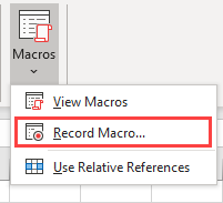
A new window will appear. Name your Macro and apply a shortcut key if you want. I’ll be using Ctrl + Shift + R as a shortcut to this Macro.

If you also want to apply this shortcut, click the little white box under the Shortcut Key and press Shift + R.

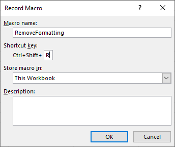
Immediately after you click the OK button, the recorder starts to record your every move. Select Table Design >> Table Styles >> More >> Clear.

Now, after the formatting is removed from the table, you can stop the recording by clicking the bottom-left corner.

Let’s see how our macro looks like.

Go to View >> Macros and click the View Macros button (Alt + F8).

From the list, select the macro and click Edit.

The code that removes formatting is just a single line. it assigns table style for a table (Table4). There is also shortcut information, you created (Ctrl + Shift + R). It’s just a comment, so you can delete it.

The code shouldn’t work just for a table with this particular name, but for the one that is currently selected.

Modify the code so it looks like this:

Now, if you run the macro or use the keyboard shortcut you created, Excel will instantly clear filters for the selected table.