Replace Special Characters in Excel

Sometimes when we import data into Excel, it may come with unnecessary special characters. We may need to replace the special characters with empty strings or other non-special characters. This tutorial shows you 6 techniques for replacing special characters in Excel.

Method 1: Use the Find & Select Option

In this method, we will use Excel’s Find & Select feature to replace special characters with empty strings.

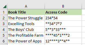
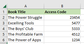
For this tutorial, let’s consider the following dataset that we have imported into Excel. The dataset has unnecessary asterisks.

We use the below steps to replace the asterisks with empty strings:

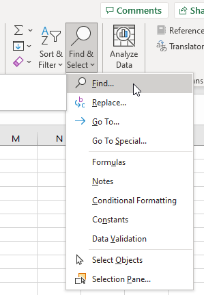
1. Click Home >> Editing >> Find & Select >> Find to open the Find and Replace dialog box.

Alternatively, you can also press Ctrl + H to open the Find and Replace dialog box.

2. In the Find and Replace dialog box that appears, type a tilde followed by an asterisk (~*) in the Find what box, leave the Replace with box blank, and click Replace All.

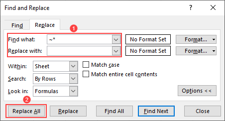
Note: The asterisk (*) is a wildcard character in Excel that represents all characters in a text string. Therefore, if you do not precede the asterisk with a tilde (~), all your data will be wiped out and replaced with empty strings.

An informational message box pops up indicating the number of replacements that have been done.

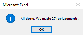
3. Click OK on the message box.
4. Click Close on the Find and Replace dialog box to close the dialog box.

The special characters in the dataset have been replaced with empty strings.

Method #2: Use the Flash Fill Feature

We can use the Flash Fill feature to replace special characters in Excel if the special characters appear in the dataset in a predictable pattern.

Flash Fill is a useful feature that fills in data automatically if it detects a predictable pattern in the data.

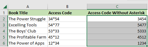
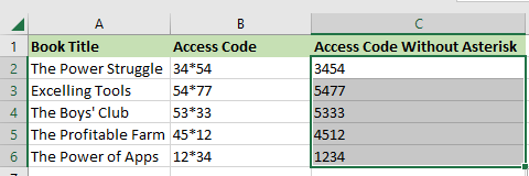
To explain how this method works, let’s consider the following dataset. Each code in column B has an asterisk after the first two numbers.

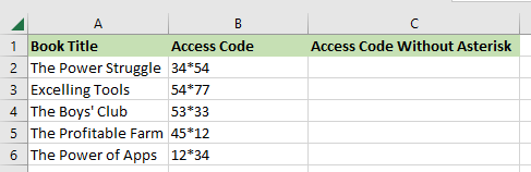
We will use Flash Fill to replace the asterisks with empty strings and display the results in column C.

We use the below steps:

1. Select cell C2 and type in the value 3454, which is the value in cell B2 without the asterisk, and press Enter.
2. In cell C3, type in the value 5477, which is the value in cell B3 without the asterisk.

As you begin to type in the second value, Flash Fill detects a pattern in the data and gives you suggestions for the next entries in grey.

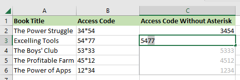
If the suggested entries are correct, press Enter to enter them.

If Flash Fill doesn’t give you suggestions for the next entries, finish typing in the second value and proceed to the next step.

3. Select the cell range C2:C6.

4. Click Data >> Data Tools >> Flash Fill.

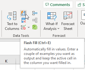
Alternatively, you can press the keyboard shortcut Ctrl + E.

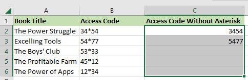
The rest of the data is automatically filled in, and the special characters have been replaced with empty strings.

Method #3: Use the REPLACE Function

We can use Excel’s built-in REPLACE function to replace special characters in Excel. This function replaces a portion of a text string with a different text string.

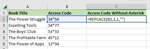
To explain how this method works, let’s consider the following dataset. Each code in column B has an unneeded asterisk character.

We will use the REPLACE function to replace the asterisks with empty strings and display the results in column C.

We use the following steps:

1. Select cell C2 and type in the following formula:

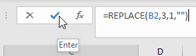
2. Click Enter on the formula bar to enter the formula.

3. Double-click or drag down the fill handle to copy the formula down the column.

The asterisks are replaced with empty strings.

Explanation of the formula

The syntax of the REPLACE function is as follows:

REPLACE(old_text, start_num, num_chars, new_text)

• The old_text is the access code in cell B2.
• 3 is the start_num or the number from which to start replacing. It is 3 because the asterisk is in the third position in the code.
• 1 is the num_chars or the number of characters we want to be replaced.
• “” (empty string) is the new_text replacing the asterisk.

Method #4: Use the SUBSTITUTE Function

We can use Excel’s built-in SUBSTITUTE function to replace special characters in Excel. This function replaces existing text with new text in a text string.

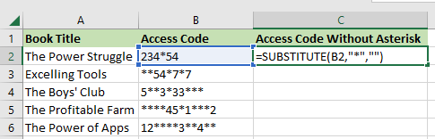
To explain how this method works, let’s consider the following dataset. Each code in column B has one or more unneeded asterisk characters.

We will use the SUBSTITUTE function to substitute the asterisks for empty strings.

We use the following steps:

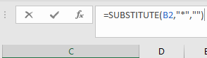
1. Select cell C2 and type in the following formula:

2. Click Enter on the formula bar to enter the formula.

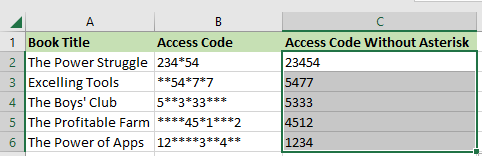
3. Drag down or double-click the fill handle to copy the formula down the column.

The asterisks have been substituted for empty strings.

Explanation of the formula

The syntax of the SUBSTITUTE function is as follows:

SUBSTITUTE(text, old_text, new_text, [instance_num])

In the formula:

• The value in cell B2 is the text containing the asterisks to be substituted for empty strings.
• The asterisk is the old_text to be substituted for the new_text.
• The “” (empty string) is the new_text.
• The instance_num is an optional argument, and therefore it was not used.

Method #5: Use a Combination of RIGHT and LEN Functions

We can apply the RIGHT and LEN functions to replace special characters in Excel. The RIGHT function returns the specified number of characters from the end of a text string, and the LEN function returns the number of characters in a text string.

You get good results in this method when the special characters in the dataset occur at regular intervals.

Suppose we have the following dataset that has asterisks at the start of each code in column B.

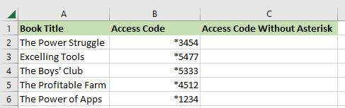
We will the combination of the RIGHT and LEN functions to extract the numbers in the codes and cut out the asterisks.

We use the below steps:

1. Select cell C2 and type in the formula below:

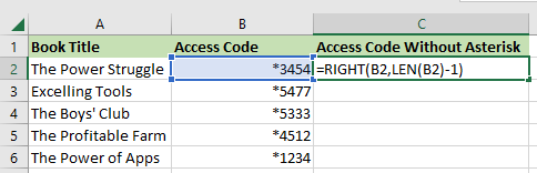
2. Click Enter on the formula bar to enter the formula.

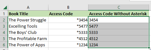
3. Double-click or drag down the fill handle to copy the formula down the column.

The asterisks have been replaced with empty strings.

Method #6: Use a User-Defined Function

We can use Excel VBA to create a User-Defined Function that we can apply to replace special characters in a dataset with empty strings.

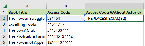
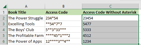
Suppose we have the following dataset that contains special characters.

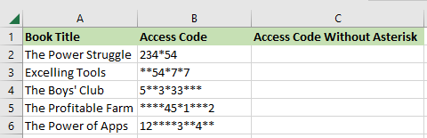
We will create a User-Defined Function that we can use to replace the special characters with empty strings.

We proceed as follows:

1. Open the worksheet that contains the dataset.
2. Click Developer >> Code >> Visual Basic to open the Visual Basic Editor.

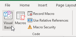
We can also open the Visual Basic Editor by pressing Alt + F11.

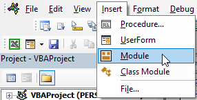
3. Click Insert >> Module in the Visual Basic Editor to insert a new module.

4. Type the following function procedure in the module:

5. Save the function procedure and the workbook as a Macro-Enabled Workbook.
6. Click the View Microsoft Excel button on the toolbar to switch to the active workbook containing the dataset.

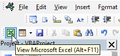
Alternatively, you can press Alt + F11 to switch to the active workbook.

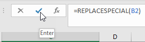
7. Select cell C2 and type in the below formula

8. Click Enter on the formula bar to enter the formula.

9. Drag down or double-click the fill handle to copy the formula down the column.

The special characters in the dataset have been replaced with empty strings.

Conclusion

This tutorial explained six techniques that can be used to replace special characters in Excel. We hope that you found the information helpful.