One of the most practical tools in Excel is certainly Pivot Tables. There are many options for users in terms of speeding up the process of everything that we do in Excel. Pivot Tables are no exception to this.
In the example below, we will show various shortcuts that can be used when it comes to Pivot Tables.
Pivot Table Shortcuts
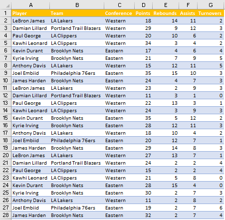
First thing first, we will create an original table, from which we will derive the data for Pivot Table. Our table will consist of NBA players and their statistics from several nights of basketball. Data shows points, rebounds, assists, and turnovers for every team, as well as the teams and conferences in which they play.
Insert Pivot Table
If we want to create a Pivot Table from this data set, we can select it, then go to Insert >> Tables >> Pivot Table >> From Table/Range. To do this with a shortcut, all we need to do is click anywhere on our data set and click ALT + N + V on our keyboard.
This is the picture that will appear on our screen:
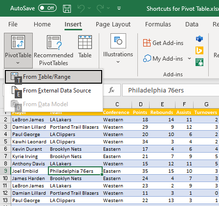
From this step, we can click either T or E on our keyboard and choose From Table/Range (T) or From External Data Source (E) option.
If we click T, we will be directed to the creation of a Pivot Table:
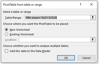
From here, we decide on the next steps.
Select Range of Pivot Table
We will create our Pivot Table with Player in Rows fields, and Sum of Points in Values Field. This is what our table looks like:

To select the entire table, we can use two shortcuts:
- The first one is a combination of CTRL + A on our keyboard.
- We can also use CTRL + SHIFT + * on the keyboard.
To make this work, we need to be located at our table. When we use one of the shortcuts listed above, our whole table will be selected:

Refresh the Pivot Tables
We can refresh either the current Pivot Table or all Pivot Tables in our Workbook. To refresh the Pivot Table that we are in, we need to select a cell in that table and then press ALT + F5.
To do this for all tables in our Workbook, we need to click CTRL + ALT + F5. For this to work, we do not need to be in a particular cell in the table.
Create a Pivot Chart from Pivot Table
There is also a very convenient option to create Pivot Chart easily from Pivot Table. For this, we need to select a cell in the table and then press ALT + F1. This is what we will get:
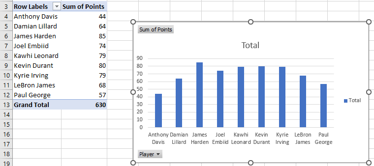
This will create a chart in the same sheet that we are currently in. To create a Chart in a new, separate sheet, we will select any cell in a table and press F11:
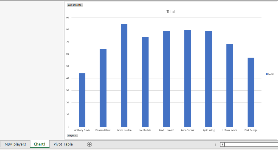
Open PivotChart Wizard
If we want to access PivotChart Wizard, which is a great tool for several options, such as Consolidate, we need to position ourselves in Pivot Table, then press ALT + D + P. Pop-up will appear:

Group and Ungroup Selected Items
You can always group two or several items in your Pivot table, to see their sum, count, or anything else you want.
To group the items with the shortcut, you need to select them, and then press Alt + Shift + Right Arrow on the keyboard. We will select the first three players in our Pivot Table, and then press the above-said combination. This is the result we have:
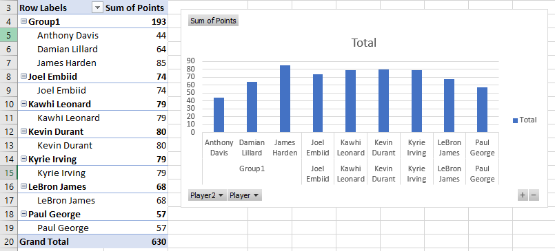
Three players will be grouped, both in Pivot Table and in our Chart. To revert the grouping, we need to choose the combination Alt + Shift + Left Arrow while selecting the same players that we grouped. This will ungroup our items.
