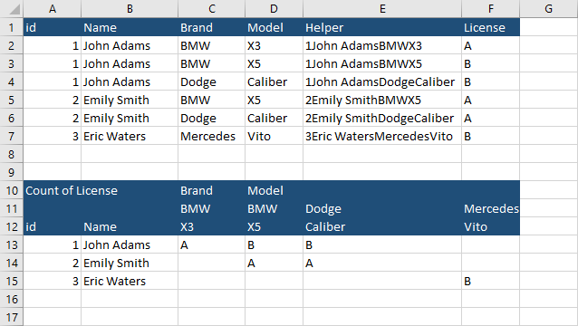
If you want to show values instead of summaries in Pivot Table, you can’t do it without any tricks, because pivot tables don’t return text, they aggregate values.
But there is a workaround that you can use to achieve a similar effect.
Show values in a pivot table using VLOOKUP
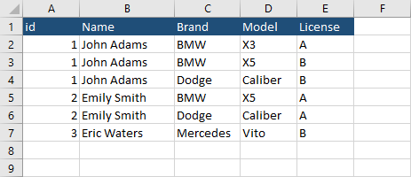
The first one uses a helper column with the VLOOKUP function.
- Create a new column, called Helper between the Model and Licence columns.
- Merge Id, Name, Brand, Model, and License inside the Helper column.

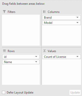
- Create a new pivot table and drag fields to the right fields.
- You should get the following pivot table.
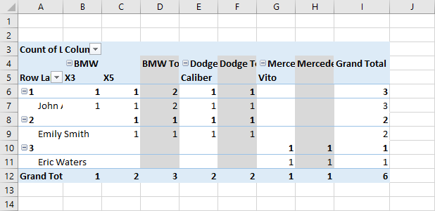
- Click the pivot table and navigate to PivotTable Tools >> Design >> Layout >> Subtotals >> Do Not Show Subtotals.
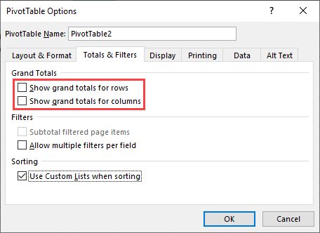
- Now, right-click the pivot table and choose PivotTable Options. Click the Totals & Filters tab. In Grand Totals, uncheck checkboxes that show grand totals for rows and columns.
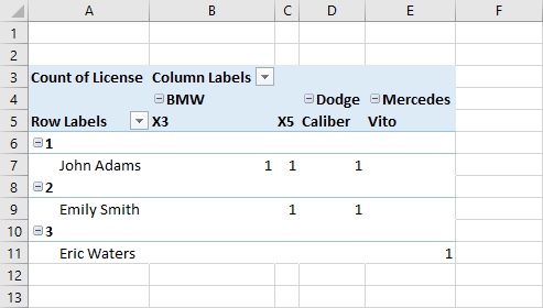
- Our example is going to look like this.
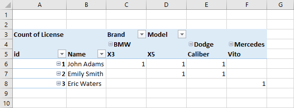
- Choose the PivotTable Options again, but this time click the Display tab and choose Classic PivotTable layout. Click Ok. This is what our Pivot Table looks like.
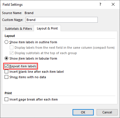
- There is one more thing to do. Right-click any car brand, and choose Field Settings. Choose the Layout & Print tab and choose Repeat item labels. Now, there are no empty fields in the brand category. It’s important to do it for our example to work.
- Select the entire Pivot Table. Copy the table and paste it as values. This will keep the layout of the Pivot Table, but remove its functionality.
- Enter this formula into cell C13: =IFERROR(VLOOKUP($A13&$B13&C$11&C$12,$E$2:$F$7,2,0),””). Be careful to enter the $ sign into the formula correctly, and see how the absolute references are preserved.
- Autofill the rest of the cells, and you will have the final example.
