We have already shown how useful the sorting options in Excel can be. However, as with pretty much every little thing in this program, anything can be done in the way in which we want, and there is always something else to be learned.
In the example below, we will show how to sort multiple rows and columns, that being just the ones that we want.
Sort Multiple Rows and Columns
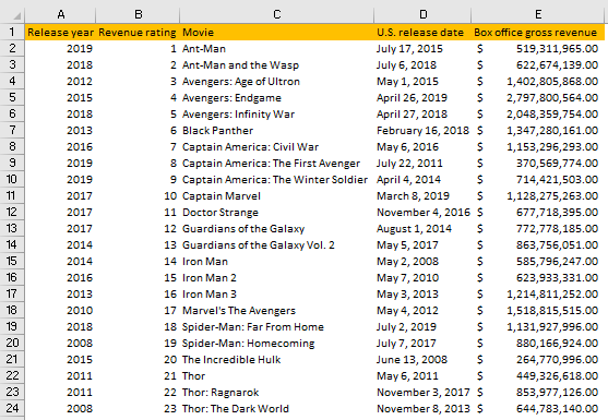
For our example, we will use the list of Marvel movies with the data of their release year, revenue rating, U.S. release year, and box office gross revenue:
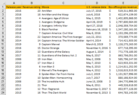
We need to point out that the data above is not constructed as a table. If we did construct it in such a way, we would not be able to use the sorting options which we will show in the following text.
Now, for example, if we want to sort only the first two columns in our data, we would select them and then go to Data >> Sort & Filter >> Sort:

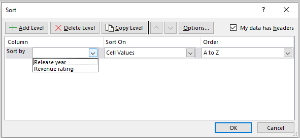
When we click on this icon above, we will be presented with a pop-up window in which we can choose the sorting between our two columns: Release year and Revenue rating:
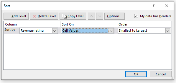
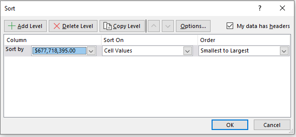
We will choose Revenue rating and choose to sort on Cell Values (other options are: cell color, font color, and conditional formatting icon), and order them from Smallest to Largest:
When we click OK, we will have these two columns changed and sorted by revenue rating, while the rest of our data (columns C:E) will remain absolutely the same:
To change the rows rather than columns, we will use the same logic. We will select range A12:E15 and repeat our steps: Data >> Sort & Filter >> Sort. We will have the following options for sorting:
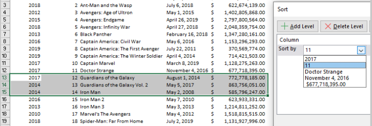
You will notice that Excel is using our first row (in our case row number 12) as the reference point and the data beneath that row (rows 13., 14., and 15.) will be affected. Since the data in row number 12 is our reference point, we can choose to sort by the data in that row, as seen in the picture above.
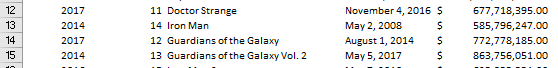
We will choose to sort our rows by the last option (movie revenue) and sort it from Largest to Smallest:
When we click OK, you will notice that our rows 13., 14., and 15. are affected and that the Iron Man movie now moved up: