Use Conditional Formatting On Errors in Excel

Applying conditional formatting on errors in Excel can help you quickly and easily identify cells that contain errors in a large dataset.

Different formatting options, for example, changing the font color or adding a fill color to cells, make the cells with errors stand out and draw attention to them. The formatting can be handy when dealing with a large dataset with many calculations, as manually searching for errors can be challenging and time-consuming.

How to Apply Conditional Formatting on Errors in Excel

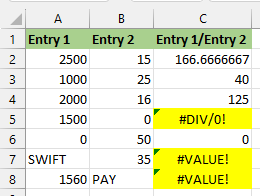
Let’s consider the following dataset with errors in column C.

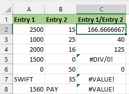
We want to use conditional formatting to highlight the cells containing errors.

We use the steps below:

1. Select the cell range C2:C8 containing errors.

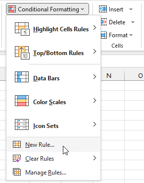
2. Click Home >> Styles >> Conditional Formatting >> New Rule.

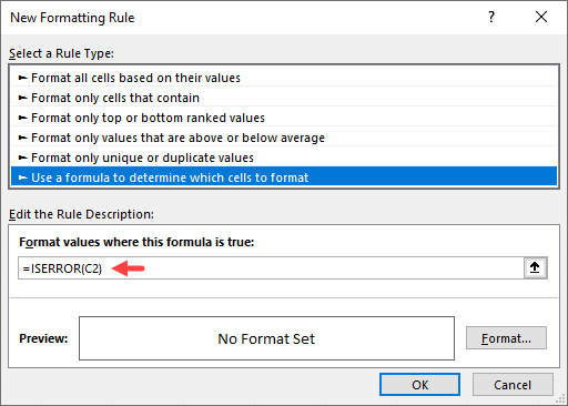
3. On the New Formatting Rule dialog box, select Use a formula to determine which cells to format on the Select a Rule Type box:

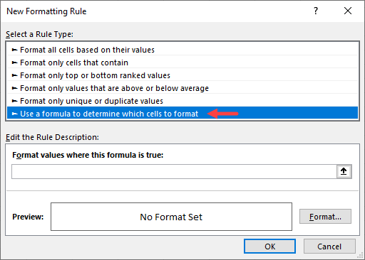
4. Enter the following formula on the Format values where this formula is true box:

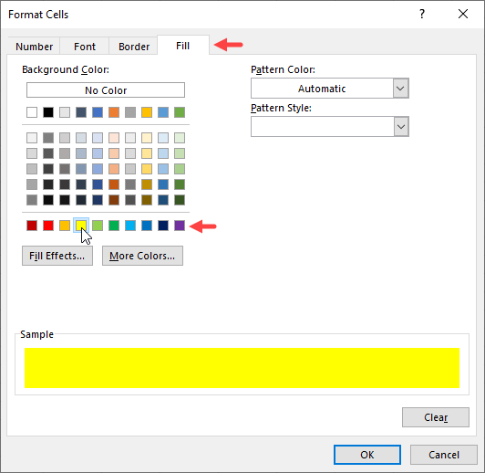
5. Click the Format button next to the Preview box.
6. On the Format Cells dialog box, open the Fill tab, choose a background color on the Background Color palette (in this example, we have chosen yellow), and click OK.

7. Click OK on the New Formatting Rule dialog box.

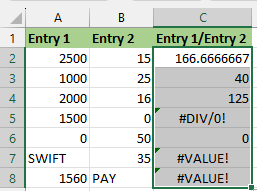
All the cells in column C which contain errors are highlighted in yellow:

Explanation of the formula

The ISERROR function checks whether a value in a cell is an error and returns TRUE if it is an error and FALSE if not.

If the ISERROR function returns TRUE, the conditional formatting feature highlights the cell containing the error. Otherwise, it leaves the cell as is.

Conclusion

Conditional formatting is a useful tool in Excel that allows you to format cells based on certain conditions. This tutorial showed the steps to apply conditional formatting to errors in Excel.

We hope you found the tutorial helpful.