Wrap Date in Excel Cell

As we work with dates in Excel, sometimes we may want to wrap dates in cells to achieve a custom visual effect.

A date in Excel is simply a number. What we see in the cell is a display format of the date.

Although we cannot wrap or split a date in a cell because it is a number, we can wrap the date display format using three methods presented in this tutorial.

Use a Custom Number Format with Ctrl + J

We can use a custom number format with Ctrl + J to wrap the display of a date in a cell by using the following steps:

1. Select the cell that contains the date value.
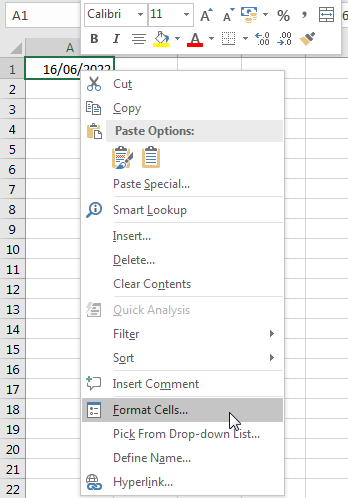
2. Right-click on the cell and click Format Cells… from the shortcut menu that pops up. We can also press Ctrl + 1 to launch the Format Cells dialog box:

3. In the Format Cells dialog box, select Custom from the Category list.
4. Delete whatever is in the Type box and type in the custom format “dddd(Ctrl + J)dd mmmm yyyy” without the quote marks. This means that we key in “dddd” without quote marks, press and hold the Ctrl key while pressing the J key and then release them, key in “dd” without quote marks, press the space bar once, and key in “mmmm” without quote marks, press the space bar once and then type in “yyyy” without quote marks.

The Ctrl + J shortcut adds a line feed.

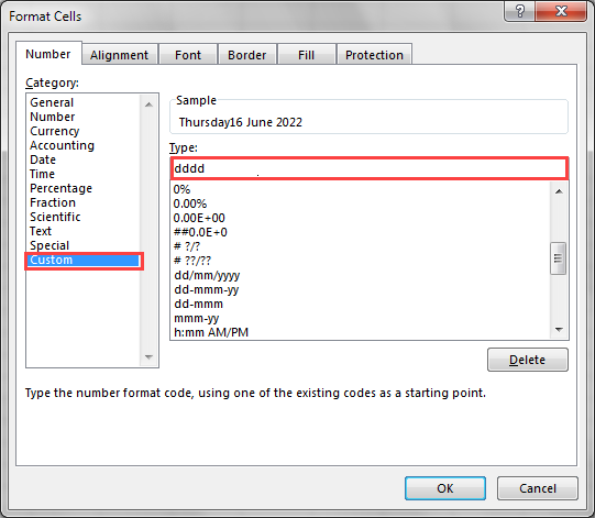
The Ctrl + J shortcut pushed some parts of the format down in the Type box and therefore we don’t see the full display custom number format but we can see the results of our typing in the Sample box.

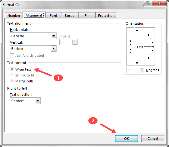
5. Click on the Alignment tab and click in the Wrap text checkbox and then click OK:

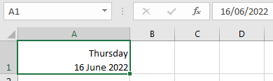
6. Manually adjust the row height and column width so that the date is fully displayed:

Use a Custom Number Format with Alt + 0010

We can use a custom number format with Alt + 0010 to wrap the display of a date in a cell by using the following steps:

1. Select the cell that has a date value that we want to format.
2. Right-click on the cell and click Format Cells… on the shortcut menu that comes up to launch the Format Cells dialog box. Alternatively, we can launch the Format Cells dialog box by pressing the keyboard shortcut Ctrl + 1:

3. In the Format Cells dialog box, choose Custom from the Category list.
4. Delete what is in the Type box and replace it with the custom format “dddd(Alt + 00100)dd mmmm yyyy” without the quote marks. This means that we key in “dddd” without quote marks, press and hold the Alt key while pressing the 0010 on the numeric keypad, key in “dd” without quote marks, press the space bar once, and key in “mmmm” without quote marks, press the space bar once and then type in “yyyy” without quote marks.

The number 0010 must be entered using the numeric keypad and not the alphanumeric keys.

The keyboard shortcut Alt + 0010 enters the line feed character and part of the format we entered looks like it disappeared but it did not disappear but it has overflowed what can be displayed in the Type box. We can however see the sample of what we have entered in the Sample box.

5. Click on the Alignment tab and select the Wrap text check box and click OK:

6. Manually adjust the row height and column width so that the date is fully displayed:

Apply a workaround that uses the TEXT function

The TEXT function converts a value to text in a specific number format.

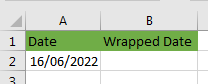
We will use the following dataset to show how this workaround can be applied:

We use the following steps:

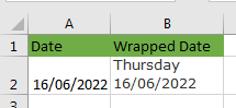
1. Select Cell B2 and type in the formula =TEXT(A1,”dddd”) & ” ” & TEXT(A1,”dd/mm/yyyy”) and press Enter key.
2. Ensure Cell B2 is still selected, right-click on it and click Format Cells… on the shortcut menu that pops up to launch the Format Cells dialog box. Alternatively, press Ctrl + 1 to launch the Format Cells dialog box:

3. In the Alignment tab select the Wrap text checkbox and click OK:

4. Manually adjust the row height and column width so that the value is fully displayed:

5. Right-click on the header of Column A and click Hide on the shortcut menu that pops up:

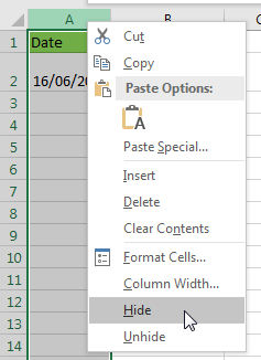
This hides Column A. If we want to do calculations based on the date we must use the value in the hidden column because what we have in Column B is not a date but text.

This workaround is best suited for the times when we are only interested in data display as in a printed copy of the worksheet but not in doing calculations based on the date values.

Explanation of the Formula

• TEXT(A1,”dddd”) – the TEXT function calculates the day of the week for the date in Cell A1 and returns the full day of the week, in this case, Thursday. If we wanted the short name of the day of the week we would use ddd, and in this case, the function would have returned Thu, the abbreviated name for Thursday.
• TEXT(A1,”dd/mm/yyyy”) – The TEXT function returns the date in Cell A1 in the specified format of “dd/mm/yyyy.”
• TEXT(A1,”dddd”) & ” ” & TEXT(A1,”dd/mm/yyyy”) – The two text strings are concatenated with a space in between using the ampersand (&) character.

Conclusion

A date in Excel is simply a number and therefore cannot be split or wrapped in a cell. What we can do however is wrap the display of a date in a cell.

In this tutorial we have looked at three methods we can use to wrap the date display format in a cell.

The methods are using a custom number format with Ctrl + J, a custom number format with Alt + 0010, and a workaround using the TEXT function.

You can use the method that best fits your situation.