How to Apply Percentage Formula in Multiple Cells in Excel

Excel is, like all computer programs, perfect for performing various arithmetic and mathematical functions.

One of these functions is to calculate a percentage of a certain number. But the real question is, how to apply the formula for percentage calculation for multiple cells?

We are going to explain that in the text below.

Percentage Formula in Multiple Cells

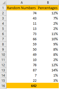
For our example, we will use a simple table of random numbers between 1 and 100.

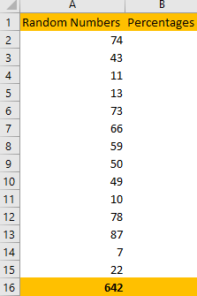
In the table above, in cell A16 we have used the formula SUM to calculate a total of the cells in the range A2:A15. Our formula is:

To calculate the percentage of a certain number in a total, we have to use the formula:

Notice that we have a $ sign surrounding both column A and row 16 in a reference to cell A16. This means that we locked the reference for this cell. Now we can drag and drop our formula to the last cell in our range, and we will have all the cells found in column A divided by grand total:

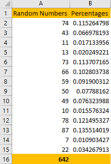
Of course, now we have to format our cells to look neater.

To do this, all we have to do is select our range and go to the Home tab >> Number, and find the percentage style shortcut as in the picture below.

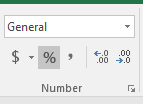
We could also select our range and use the shortcut key: CTRL + SHIFT + % (% sign is usually number 5 on your keyboard).

Once we do this, our table looks like this:

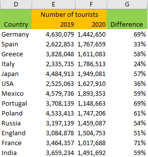
Of course, locking of grand totals is not always necessary. Let’s say that we have a table with the number of tourists (totally random) in various countries in 2020 and 2021.

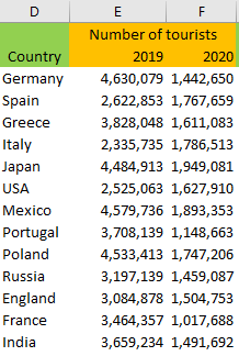
As expected, due to COVID-19, the number of tourists in 2020 is significantly lower in all countries in comparison with 2019. Again, totally random figures.

To calculate the difference in percentages between these two years, we will input the simple formula in cell G3:

This formula calculates:

We will drag this formula to the last row and we will format column G to be in percentages, as we did with the example above.

Our table will look like this: