In Excel, two functions are designed in a way to work with these types of codes: CHAR and CODE. If you want to find a character according to its ASCII number, you should probably use the CHAR function.
If you want to return the ASCII number for a certain character, you should probably use a CODE function.
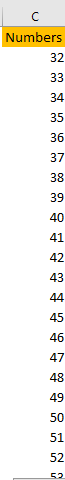
Now, knowing all of this we will first make a list of numbers from 32 to 126.
To do this, we will use the following formula:
|
1 |
=SEQUENCE(127-32,,32) |
This formula will give us the range of numbers from 32 to 126, and it starts with the number 32.
It will look something like this in our Excel table:
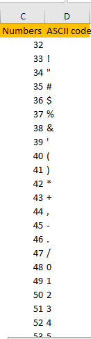
Now, we did say that the formula for converting these numbers into ASCII codes is CHAR, so we will input that formula in cell D2:
|
1 |
=CHAR(C2) |
And drag it till the end of our range (in this particular case cell D96):
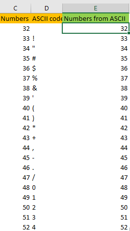
Now we have ASCII codes for these numbers. Just to prove this works the other way around as well, we will put the following formula in cell E2:
|
1 |
=CODE(D2) |
This is what we end up with:
Now let us say that we have a word written in cell A2: “HOME”.
To find the ASCII code for each letter of this word, we will use the VLOOKUP function, and we will concatenate the letters.
We will put a formula in cell B2 and it will go like this:
|
1 |
=VLOOKUP("H",D:E,2,0)&"_"&VLOOKUP("O",D:E,2,0)&"_"&VLOOKUP("M",D:E,2,0)&"_"&VLOOKUP("E",D:E,2,0) |
As you can notice, our formula searches for the value that we define (letters “H”, “O”, “M”, and “E”) by looking at columns D and E. We search for the value in column D and we then return the value that is located next to it in column E.
We also added “_” so that we could distinguish what are the values for every letter.
This is our result:
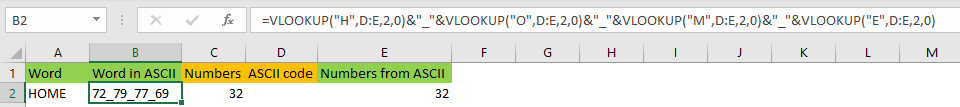
We can see that the corresponding number for the letter “H” in ASCII is number 72, 79 for „O“ and so on.