A lot of times, people are giving up on Excel because they have problems with formatting. One of the most common problems is formatting time.
In the example below, we will show how to convert our cell or range to time, when we have the same time stored in a string variable. Then we will use another example for the same exercise, but to format the date, not just the time.
Convert Time String to Time
It is very important to understand that for Excel, time is observed simply as a number. For example, number 1 represents the oldest date in Excel, which is 1/1/1900. If we have our number stored in a string, the first thing that we need to do is convert it to a number.
Let us say that we have the following time values in our workbook:

From these numbers above, we would like to have a proper time, for example, we would like the first cell to be equal to 18:10, or 6:10 PM.
Our first job is to convert string numbers into time value numbers. To do so, we will use the formula:
|
1 |
=TIMEVALUE(LEFT(A2,LEN(A2)-2)&":"&RIGHT(A2,2)) |
The TIMEVALUE function serves for converting time presented as text into Excel time. The rest of the function makes sure we return one or two characters of the string, depending on the total number of characters, adds a “:” sign, and returns two characters that are located on the right side of the string.
As a result, we get the following numbers:
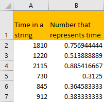
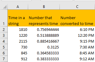
These numbers in column B are nothing but the numeric representation of the time that is stored but „hidden“ in column A. We will copy and paste values from column B to column C, select the values in column C that we want to format, go to the Home tab and click on the button in the bottom right corner next to Number:
 On the pop-up window that appears, we will choose Time, and select an option that we prefer:
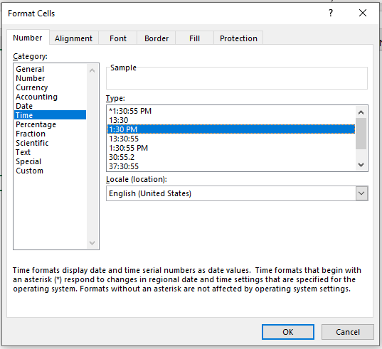
In our case, we will choose option number 3, which is an option to show AM or PM for the hours. You can already see that our numbers are converted to time values.
When we click OK, our table looks like this:
Convert Date and Time String to Date and Time
When we have date and time written as a string, we can also use a formula to help us convert our string to something senseless, i.e. to a proper date and time formatting.
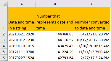
Let us say we have the following numbers in a string:
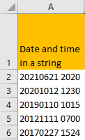
We can see that number in cell A2 represents the 6th of June of 2021, and the time is set to 20:20.
But we need to convert this into this said date and time. To achieve this, we will use the formula below:
|
1 |
=DATE(LEFT(A2,4),MID(A2,5,2),MID(A2,7,2))+TIME(MID(A2,10,2),RIGHT(A2,2),0) |
This formula first finds a date, using the LEFT formula and four digits from the left side for a year, MID formula for finding month and day, while starting from the fifth and seventh value in the string, and taking two values for month and two for the day.
Then, the formula finds time, and takes hours from the MID formula, starting from the 10th value in our string, and taking two numbers. Then it uses the RIGHT formula to find minutes and takes two values.
Formulas LEFT, MID and RIGHT are usually used to derive a certain value from a string, and the formula above shows it in a very good way.
Once we insert our formula in cell B2 and drag it to the end of our table, we get the following results:
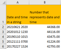
We will copy these numbers into column C, select the values, and then go to formatting options again and choose a date with time option:
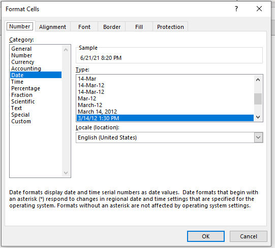
Once we click OK, we will see desired results:
