Find and Replace
The easiest way to find multiple values in Excel is to use the Find feature.
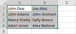
First, select the cells you want to be searched.
Then navigate to Home >> Editing >> Find & Select >> Find. You can also use the Ctrl + F keyboard shortcut for quick access.
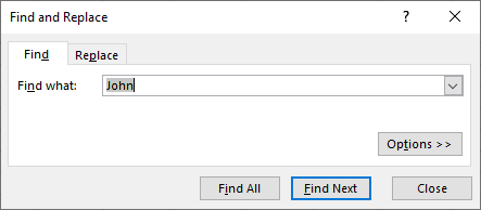
Click the Find All button to search the entire selected area. It will show a list of cells meeting the criterion.
Without doing anything else, press Ctrl + A shortcut to select all of them.
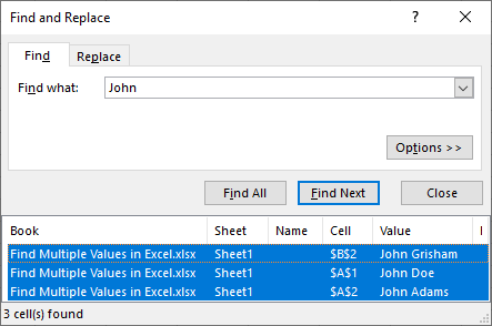
Click Close.
Now, instead of all the previously selected values, only three cells are selected – the ones with the phrase “John”.
If you click Options >>, before clicking Find All, you can find additional settings, for example, you can force Excel to search text that matches the case.
FILTER Function for Excel 365
The VLOOKUP function is very useful if you want to find a value based on a lookup value. It only works for unique values. If the are duplicates, the function will return only the first of them.
So, if the table contains multiple lookup values, this function is not going to work.
If you want VLOOKUP functionality with multiple values, you can use the FILTER function. It is extremely easy to use.
This function is only available for Excel 365 subscribers, so if you are using a different version of Excel, it’s not going to work for you.
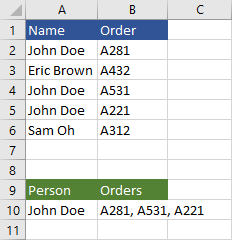
Let’s see how it looks like using this example:
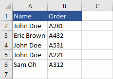
Now, we are going to display all orders of John Doe.
First, let’s use the VLOOKUP function. Insert this formula into cell B10.
|
1 |
=VLOOKUP(A10,A2:B6,2,FALSE) |
The formula returns the first John Doe’s order on the list.
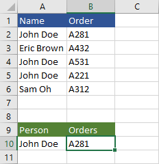
But two other orders should be included.
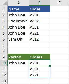
Now, let’s use the FILTER function.
Insert the new formula into cell B10:
|
1 |
=FILTER(B2:B6, A2:A6=A10) |
This is the result:
It’s very easy and fun to use, but it’s not available in the previous versions of Excel. Let’s find out how we can create a formula that works similarly for someone who doesn’t use Excel 365.
INDEX function
We are going to use the INDEX function to achieve a result similar to that of the FILTER function. Enter this formula in cell B2:
|
1 |
=INDEX($A$1:$B$6,SMALL(IF($A$1:$A$6=$A$10,ROW($A$1:$A$6)),ROW(1:1)),2) |
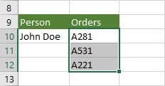
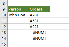
This formula returns the first occurrence of John Doe’s order: A281.
If you Autofill the remaining cells you are going to get the remaining orders.
Let’s break this formula into smaller pieces:
|
1 |
=IF($A$1:$A$6=$A$10,ROW($A$1:$A$6)) |
If a cell in range A1:A6 equals A10 (John Doe), then it returns row number, otherwise, it returns FALSE.
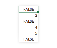
2, 4, and 5 are the rows where the name “John Doe” is present.
The next part of the formula uses the SMALL function, which returns the n-th smallest value.
|
1 |
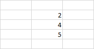
=SMALL(IF($A$1:$A$6=$A$10,ROW($A$1:$A$6)),ROW(1:1)) |
ROW(1:1) returns the first row. If you use the Autofill, it’s going to return 1, 2, 3, etc. row number.
The formula will return the numbers: 2, 4, and 5.
The INDEX function returns the value at a given position.
|
1 |
=INDEX(array, row_number, column_number) |
The array is a range A1:A6. Row numbers are 2, 4, 5. The column number is 2.
|
1 |
=INDEX($A$1:$B$6,SMALL(IF($A$1:$A$6=$A$10,ROW($A$1:$A$6)),ROW(1:1)),2) |
If you enter these formulas, you are going to get the same result:
|
1 2 3 |
=INDEX($A$1:$B$6, 2, 2) =INDEX($A$1:$B$6, 4, 2) =INDEX($A$1:$B$6, 5, 2) |
Getting rid of errors
If you try to Autofill these values beyond matching elements, you are going to get the #NUM! error.
To fix it, you have to use this formula, that deals with this problem:
|
1 |
=IF(ISERROR(INDEX($A$1:$B$6,SMALL(IF($A$1:$A$6=$A$10,ROW($A$1:$A$6)),ROW(1:1)),2)),"",INDEX($A$1:$B$6,SMALL(IF($A$1:$A$6=$A$10,ROW($A$1:$A$6)),ROW(1:1)),2)) |
You can learn more about the index function and how you can use it to return multiple results, read article on this subject.
Multiple values in a single cell
If you prefer to have all orders inside a single cell, separated by a comma, you can do it by creating a formula that contains both the FILTER and TEXTJOIN functions.
TEXTJOIN joins a range of text strings inside a single cell.
Insert this formula to cell B10:
|
1 |
=TEXTJOIN(", ", TRUE, FILTER(B2:B6, A2:A6=A10)) |
This is how the result looks like: