If you are dealing with Excel, you will certainly stumble upon arrays at some point in time. Excel arrays are structures that can hold a collection of values.
In the example below, we will show how to get the value that we want from 2-dimensional arrays.
Get Value from 2D Array
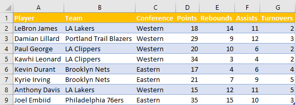
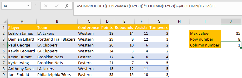
For our example, we are going to use a table of NBA players and their statistics for several nights, including points, rebounds, and turnovers:
Now, if we want to find out the location of any value of our values in terms of its rows and columns, we can use the following formulas:
|
1 |
=SUMPRODUCT((data=FORMULA(data))*ROW(data))-ROW(array)+1 |
|
1 |
=SUMPRODUCT((data=FORMULA(data))*COLUMN(data))-COLUMN(data)+1 |
Array in this case represents the cells from which we want to derive our data.
Our goal is to find the column and row number for any given value. What the formula above does, is that it uses any formula that we want (MIN, MAX, or similar), and compares our data to this value. Then we get an array of TRUE and FALSE results. When we get these results, we multiply them by the result of ROW (or COLUMN) and an array of row numbers. At the and, we add the number 1 to get an index that is relative to our named array.
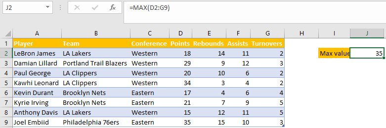
We will use this formula to try to find the MAX value for the range D2:G9.
To find out the minimum value of this range, we will input the following formula in cell J2:
|
1 |
=MAX(D2:G9) |
We can see that that value is 35:
Now we want to find the location of this value (to which column it belongs and to which row).
First, we will find the row value by using the following formula:
|
1 |
=SUMPRODUCT((D2:G9=MAX(D2:G9))*ROW(D2:G9))-ROW(D2:G9)+1 |
We are using this formula to find the max value of our range, and we produce multiple checks for true and false. Once we input this formula, we will get the following result:
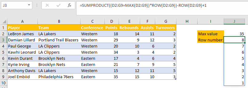
You will notice that we will get the number 8 as our result, which is correct. You will also notice that we have a bunch of other numbers created beneath, all the way up to number 1.
This is called spill behavior. It is automatic and native, and in Office 365 any formula can spill results. Spilling cannot be disabled with some global settings.
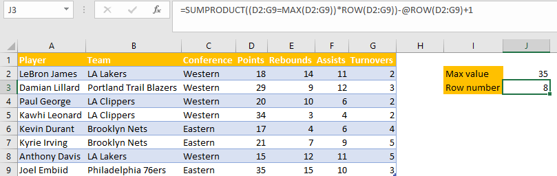
To ensure that it does not appear in our example, we will input the “@” sign in our formula, right behind the “=” sign. We will then click ENTER and get the following results:
Now, to get the column number, we will use the following formula:
|
1 |
=SUMPRODUCT((D2:G9=MAX(D2:G9))*COLUMN(D2:G9))-COLUMN(D2:G9)+1 |
We will also add a “@” sign in front of our formula, and will have the following results in our table:
We now have the exact location of our desired cell (max value in our range) that represents a cell in the eighth row and first column, i.e. cell D9.
Get Corresponding Column for Value in Array
If we want to find out to which column in our array our value belongs, we can use the following formula:
|
1 |
=INDEX(array,1,SMALL(IF(NOT(ISERROR(SEARCH(desired cell, array))),COLUMN(column that are included),99^99),1)) |
We know that our array will be our whole table. We want to find in which column the word „LeBron James“ is located, and we will put his name in cell L2. Our formula will look like this:
|
1 |
=INDEX($A$1:$G$9,1,SMALL(IF(NOT(ISERROR(SEARCH(L2,$A$1:$G$9))),COLUMN($A:$G),99^99),1)) |
When we put this formula into the cell M2, it will look like this:
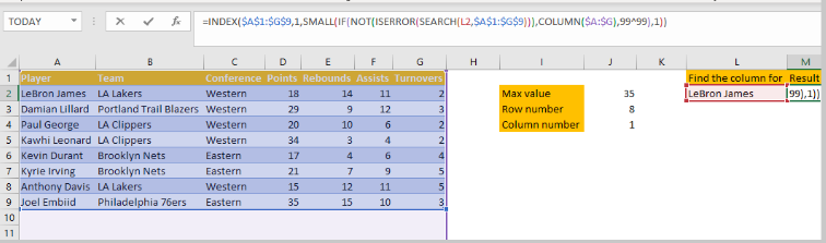
And we will have our desired result:
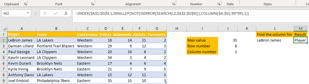
To simply explain it, the above formula does the following:
- It uses the SEARCH function to find if any entries in our range are equal to cell L2. This formula produces an array of values.
- It then uses IF and NOT to find the column number if we find the match. Otherwise, it returns a very high number (99^99).
- Then we use the SMALL function to retrieve the lowest column number where we have a match.
- Now when we have the column number we will use the INDEX function in the end to retrieve the value.