Depending on the data you have in your worksheet you may use one of the following ways to highlight duplicate rows.
Highlight duplicate rows in one column
The first one is the most basic. Here, we have only one column, so when we highlight a single cell, we also highlight a single row.
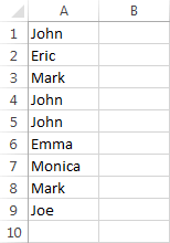
To highlight duplicate rows, first select cells from A1 to A9.
Go to HOME >> Styles >> Conditional Formatting >> Highlight Cells Rules and select Duplicate Values.
A new window will appear.
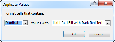
Make sure that you’ve selected Duplicate and click OK.
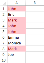
All rows which are duplicates are now highlighted.
Check multiple columns
We can’t use the above method if we want to check duplicates by rows, that have more than one column.
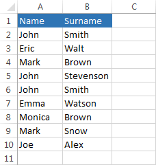
In the above example, each row consists of two columns. So Excel has to take into consideration both Name and Surname.
Let’s create another column where we merge both columns and call it Merged.
Enter the following formula in cell C2.
|
1 |
=CONCATENATE(A2,B2) |
Use autofill to fill the rest of the cells and press F9 to refresh the workspace.
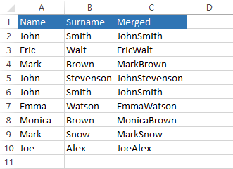
Now, when we use HOME >> Styles >> Conditional Formatting >> Highlight Cells Rules >> Duplicate Values…on column C only this column will be highlighted.
In order to highlight all columns (A, B, and C), we have to use rules.
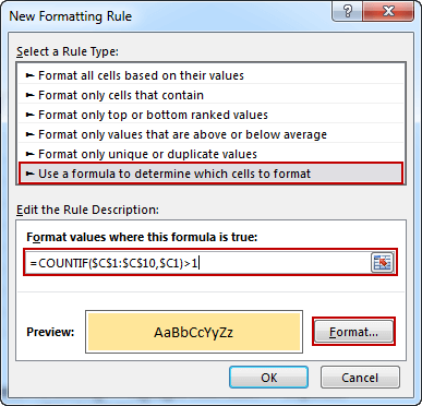
- Select cells from A1 to C10.
- Go to HOME >> Styles >> Conditional Formatting and click New Rule….
- Click Use a formula to determine which cells to format.
- Click the Format… button to choose a color.
- Enter the following formula: =COUNTIF($C$1:$C$10,$C1)>1.
- Click OK.
This is the final example.
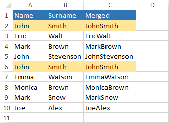
Formula analysis:
The COUNTIF function takes two arguments:
Range:
|
1 |
=COUNTIF($C$1:$C$10, $C1)>1 |
Criteria:
|
1 |
=COUNTIF($C$1:$C$10, $C1)>1 |
As you can see the criteria is $C1. There is no dollar sign in front of number 1. That means that the row number is not absolute. In other words, we check each criterion (C1, C2, …, C10) and compare it to the range (C1:C10).
Read this lesson if you want to learn more about absolute and relative cell references.
