If you have been using Excel at any point, you have certainly heard of the VLOOKUP function. Now, although this function is pretty valuable, there are two functions that combined together, are proven to be even more powerful and useful.
However, people tend to use them less, mostly because of the lack of understanding. These functions are INDEX and MATCH.
We will explain each one separately, and then, since they work best together, show their joint functioning. In the end, we will show the use of these functions to derive data from the table in a very simple way.
For our examples, we will use the list of Marvel movies that were released so far.
Index Function in Excel
The Excel INDEX function returns the value at a given position in a range or array.
The syntax of this function is as follows:
|
1 |
=INDEX(array, row_num, [col_num], [area_num]) |
Arguments are:
array – A range of cells, or an array constant.
row_num – The row position in the reference or array.
col_num – [optional] The column position in the reference or array.
area_num – [optional] The range in reference that should be used.
Don’t get confused by this. We will explain everything in an example. Let’s say that we have a list of Thor movies, their budget, and U.S. release date, like in the picture below:

If you want to find out what was the budget of Thor: Ragnarok, you can use the INDEX function.
We can see easily that the budget of Thor: Ragnarok is located in cell B3, so we will use this information to „hard code“ our function.

Our function is located in cell E2 and goes:
|
1 |
=INDEX(A1:C4,3,2) |
We used the whole table for our array, i.e. range A1:C4. Since the desired data is found in row number 3, we used this number for row_num, and our column_num is number 2, as the budget is located in column B.
It is worth mentioning that we hard-coded our row and column numbers, meaning that we just placed two numbers that we knew will give us the correct data.
Having all this in mind, if you would assume that the INDEX function does not seem so helpful at all, you would probably be right. Its real power can be seen in combination with the MATCH function.
Match Function in Excel
The definition of the MATCH function could be that this function searches for a specified item in a range of cells and then returns the relative position of that item in the range.
Its syntax is:
|
1 |
=MATCH(lookup_value, lookup_array, [match_type]) |
Arguments are as follows:
lookup_value: This is a required field. The value that you want to match in lookup_array. In our example, it could be the name of the movie that we want to find. The lookup_value argument can be a value (number, text, or logical value) or a cell reference to a number, text, or logical value.
lookup_array. Also required. The range of cells being searched.
match_type. This is an optional field. It can have three values: -1, 0, or 1. The match_type argument specifies how Excel matches lookup_value with values in lookup_array. The default value for this argument is 1. In our example, we will use the value 0, which is the exact value of the lookup_value.
We used the same example as before to show the use of the MATCH function:
|
1 |
=MATCH("thor",A1:A4,0) |

In this example, we are searching for the word „thor“ (lookup_value), in range A1:A4 (lookup_array), and we are searching for the exact word (our match_type is 0). Our final result is number 4, which is the row in which our value is found.
Notice that the MATCH function is not case sensitive as the function returned the value although we did not input capital the letter “T“.
If we change our match_type to 1, however, we will get different results.
As seen, the result in our cell E3, for the function:
|
1 |
=MATCH("thor",A1:A4,1) |
is 1. This is because match_type 1 finds the largest value that is less than or equal to our lookup_value, not the exact value, as match_type 0 does.

Match_type 1 is also a default value, so if you leave this argument undefined or you omit it, it will always return this value for the argument.
Index and Match Together
To fully appreciate these two abovementioned functions, we need to see how they work together.
Let’s say that we want to find the budget for Thor: Ragnarok with this function. Our function would be as follows:
|
1 |
=INDEX(A1:C4,MATCH("Thor: Ragnarok",A1:A4,0),2) |

We first started with the INDEX function and we declared our array (the whole table), then, instead of „hard-coding“ the row that we need we decided to use the MATCH function and to find „Thor: Ragnarok“ (lookup_value) in range A1:A4 (lookup_array). We also chose 0 as our match_type.
Finally, we defined our column_value as number 2. We did not use the MATCH function for columns, but we can do this as well, and we will see this in the next example.
Index and Match with Excel Table
To show the full power of the Index and Match working together, we are going to use the table with all the Marvel movies that were released so far (table below).
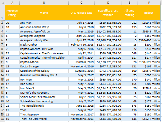
These movies are in alphabetical order. We have a total of six columns and a total of 23 movies.
Our reference point (primary cell) will be the Revenue rating. This column refers to the revenue that certain movie has in comparison with other Marvel movies.
In column H we will copy all the data from the first row, and we will do this with the TRANSPOSE option.
First, we select all the data from the first row- range A1:F1. Then we click the right mouse click and choose the option Copy. We can use the keyboard too after the selection. For this option, we use the shortcut CTRL+C.

When we do that, we go to the cell where we want to paste our data to. In this case, we go to cell H1 and click our right mouse button.
We will be shown a lot of paste options. The one that we should choose is usually in the fourth place, and has the icon as marked in the picture below:

When we finish this up, we should have our rows from the table lined up vertically in column “H”.
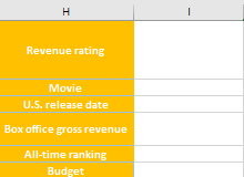
For our example, we will input our data into column I. Since Revenue rating is our reference point, we can input any number between 1 and 23 (total number of movies).
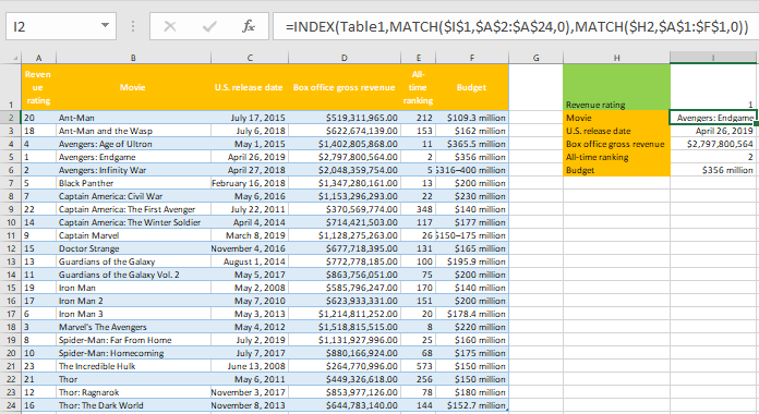
In cell I2, we will input our INDEX MATCH function, and it will be:
|
1 |
=INDEX(Table1,MATCH($I$1,$A$2:$A$24,0),MATCH($H2,$A$1:$F$1,0)) |
We will explain this function one step at a time (bold text is for the part of the function that is being explained):
=INDEX(Table1– this is our array. Since we created our list of movies as a table (we left the name of table Table1- this is a generic name for the first table created in the Excel file. If we create another one, the table name will be Table2). Our array will remain the same in all columns since we derive all the data from this table.
=INDEX(Table1,MATCH($I$1,$A$2:$A$24,0)- Next thing, we have to define our row_num. We do this with the help of the MATCH function and our reference cell, which is cell I1. Cell I1 is our lookup_value in this case. Our lookup_array is the range A2:A24 i.e. the revenue ratings of the Marvel movies.
Do not get confused by the “$“ sign. This sign in an Excel cell reference affects just one thing – it instructs Excel how to treat the reference when the function is moved or copied to other cells. In our case, both the row and the column are „locked“ for cell I2, and our lookup_array.
So far, our function means that Excel will look into our whole table, and it will search in the range A2:A24 for the value that we input in cell I2. From our table, it is clear that Excel will return the value from row number 5 in column A.
|
1 |
=INDEX(Table1,MATCH($I$1,$A$2:$A$24,0),MATCH($H2,$A$1:$F$1,0)) |
For the last part, we defined the column for our INDEX function. We used the MATCH function for this one more time. In this case, our lookup_value is in cell H2, which corresponds to the value “Movie”.
You can notice that we have only the dollar sign in front of the letter H, meaning that we “locked” only the column value, not the row value. When we copy-paste this function into a different cell, the value of the row will change. For example, if we copy-paste this function into the cell I3, all the values will be the same but the value for lookup_value in this MATCH function will be H3.
Our lookup_array in this case is the range A1:F1. Those are our column title values.
With this part of the function, Excel will look into our whole table, and it will search in the range A1:F1 for the value that we input in cell H2. From our table, it is clear that Excel will return the value from column B.
For the final part, the beauty of everything we have done so far can be seen if we just copy-paste our cell I2 into cell I3. We will get the function as seen in the picture below, which means that we will get the exact release date in the U.S. for the movie Avengers: Endgame.
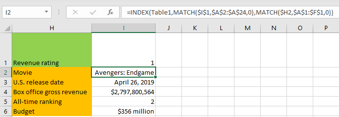
In the same way, we will get all data below. We just need to copy-paste our cell I2 into all the cells in range I4:I6.
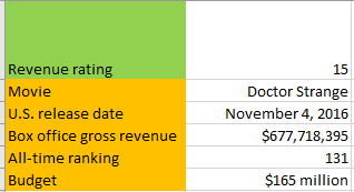
If we want to find out what the movie is, let’s say, 15th in terms of revenue from all the Marvel movies, and all the data for this movie, we just type the number 15 into cell I2. We do not have to do anything else.
