When you want to look up a value in a table based on another cell, you can use the VLOOKUP function. But there is a problem with this function. It returns only one result even if more meet the criteria.
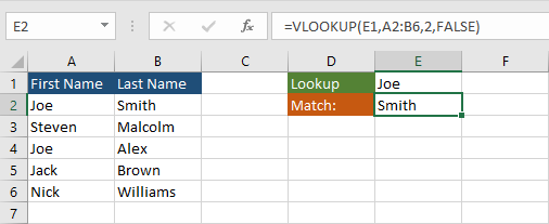
Take a look at the following example.

Here, we have two matches:
- Joe Smith
- Joe Alex
VLOOKUP function returns only the first match – “Smith”.
Returning multiple matches and displaying them vertically
If you want to return more than one value, you have to use array formulas. Array formulas are designed to work with a series of cells, rather than a single cell.
Enter the following formula into cell E2 and press Ctrl + Shift + Enter to convert it into an array formula.
|
1 |
=IF(ISERROR(INDEX($A$1:$B$6,SMALL(IF($A$1:$A$6=$E$1,ROW($A$1:$A$6)),ROW(1:1)),2)),"",INDEX($A$1:$B$6,SMALL(IF($A$1:$A$6=$E$1,ROW($A$1:$A$6)),ROW(1:1)),2)) |
Autofill the few cells down.

You are going to get additional results if there are any.

As you can see, there are two matches inside our example.
Code explanation
Let’s break down the formula to understand what it does. It’s modified to work with normal formulas
|
1 |
=IF(A1=$E$1,ROW(A1)) |
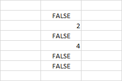
If you autofill the rest of the results, you are going to get the row numbers, where the value meets the criteria. If it doesn’t meet the criteria it returns FALSE.

Now, imagine that you do it not, row by row, but for all rows at once. That’s why you are going to use an array formula. Enter the formula and press Ctrl + Shift + Enter.
|
1 |
=SMALL(IF($A$1:$A$6=$E$1,ROW($A$1:$A$6)),ROW(1:1)) |
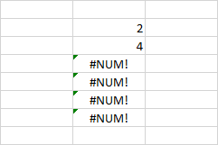
you are going to get this result.

The SMALL function takes two arguments: an array of values and the nth lowest value.
If I have the following values: 1, 1, 2, 3.
=SMALL(array,2) returns 1 because the smallest value is 1, but the second smallest is also 1.
=SMALL(array, 4) returns 3 because it’s the fourth smallest value.
When you autofill the formula, in the first one you will have ROW(1:1). In the second ROW(2:2). The ROW function returns the row number. In other words, this works as an incrementation – 1, 2, 3, etc.
Now, take a look at how the IF function works in our example. That takes the first lowest value ROW(1:1) which is 2, and the second lowest value ROW(2:2) which is 4. And this is what our example looks like.
Next, let’s analyze the INDEX function. It takes a range and returns the value under given row and column numbers.
Here, is an example.
|
1 |
=INDEX(A2:B6,3,2) |
Will return “Alex”. This is the value under the third row of this range (which is row 4 because it starts from A2, not A1) and the second column.
Now, take a look at our formula.
|
1 |
=INDEX($A$1:$B$6,SMALL(IF($A$1:$A$6=$E$1,ROW($A$1:$A$6)),ROW(1:1)),2) |
It takes a range as the first argument, and values from the small function, which are 2 and 4 as rows, and 2 as columns. Therefore the function returns the first value under row 2 and column 2 (B2), and row 4 and column2 (B4), which are “Smith” and “Alex”.
|
1 |
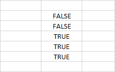
=ISERROR(INDEX($A$1:$B$6,SMALL(IF($A$1:$A$6=$E$1,ROW($A$1:$A$6)),ROW(1:1)),2)) |
The ISERROR function returns TRUE if there is an error in the formula.

Now, take a look at the full formula.
|
1 |
=IF(ISERROR(INDEX($A$1:$B$6,SMALL(IF($A$1:$A$6=$E$1,ROW($A$1:$A$6)),ROW(1:1)),2)),"",INDEX($A$1:$B$6,SMALL(IF($A$1:$A$6=$E$1,ROW($A$1:$A$6)),ROW(1:1)),2)) |
If the result is TRUE, enter the blank value (“”), otherwise insert the result from the INDEX function, which is “Smith” and “Alex”.
