INDEX and MATCH with the LARGE Function in Excel

Finding cells that meet multiple criteria is a common task in Excel. In this tutorial, we look at how to use the combination of INDEX, MATCH, and LARGE functions in Excel to find specific data in a dataset.

We first describe and explain how each function works.

Combination of INDEX, MATCH, and LARGE functions

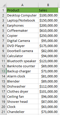
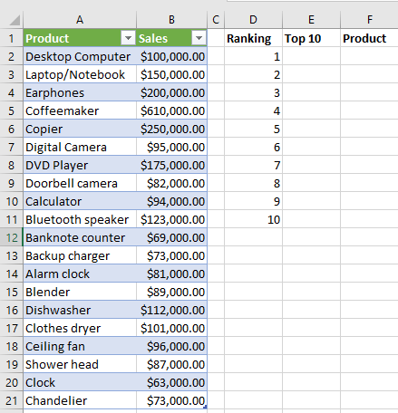
We use the following dataset of product sales to explain how the combination of INDEX, MATCH, and LARGE functions can be used to pull data that meets certain conditions from the top of a dataset:

We recommend that you first convert the data range to a table using the steps below:

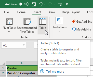
1. Select the whole dataset and click Insert >> Tables >> Table.

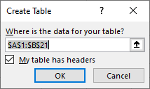
2. Ensure that the defaults in the Create Table dialog box are correct and click the OK button.

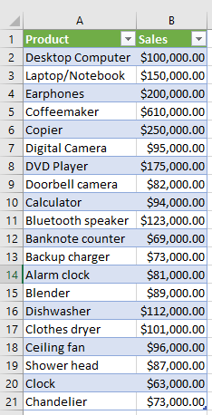
The data range is converted to a table:

We want to find out the top 10 best-performing products from the table. We proceed as follows:

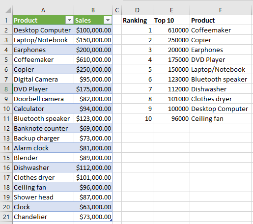
3. Type Ranking, Top 10, and Product in cells D1, E1, and F1 respectively. Type values 1 to 10 in range D2:D11. Your dataset should look like the one below:

4. Select cell E2 and type in the following formula:

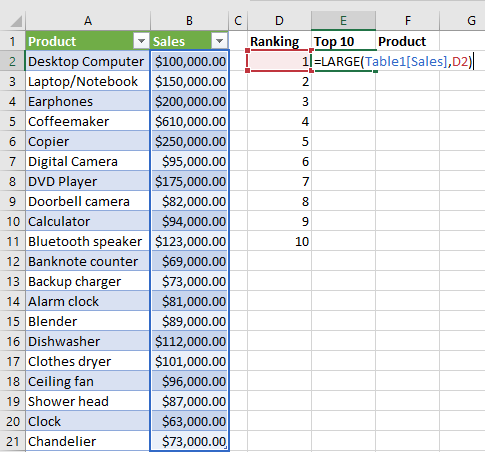
5. Press the Enter key and double-click or drag down the fill handle to copy the formula down the column.

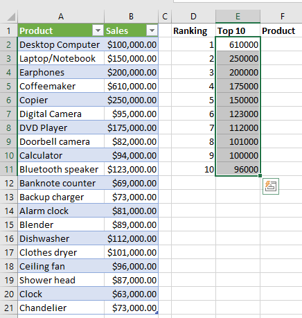
We get the sale amounts of the 10 best-performing products.

We need to find out the products associated with the amounts.

6. Select cell F2 and type in the following formula:

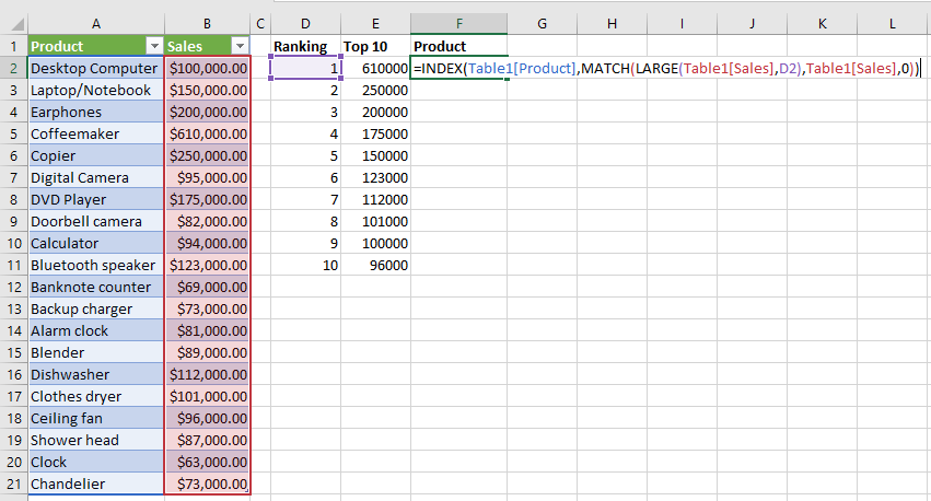
7. Press the Enter key and double-click or drag down the fill handle to copy the formula down the column.

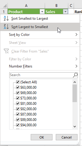
8. Click the down arrow in the Sales header and click Sort Largest to Smallest:

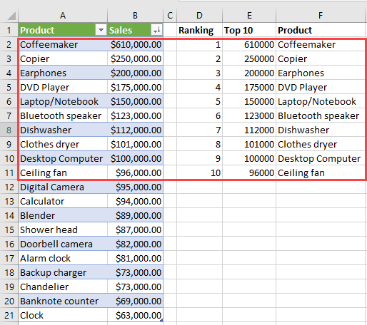
The results confirm that the formula returned the correct values:

Explanation of the formula

• Table1[Product]. Look for the product in the Product column.
• MATCH(LARGE(Table1[Sales],D2),Table1[Sales],0. Find the largest value in the Sales column in the position in cell D2 and match it to the product indexed in the Product column.

INDEX Function

The INDEX function returns a value or the reference to a value from within a table or a range.

It has two forms:

• The array form that returns the value of a specified cell or array of cells
• The reference form that returns a reference to specified cells.

Array form

The array form of the INDEX function returns the value of an element in a table or an array selected by the row and column number indexes.

Use this form if the first argument to INDEX is an array constant.

Syntax:

INDEX(array, row-num, [column_num])

The function has the following arguments:

• array. It is required. It is an array constant or a range of cells.

Note: If the array contains only one column or row, the corresponding column_num or row_num argument is optional. If the array has more than one row or column, and only the row_num or column_num argument is used, an array of the entire row or column is returned.

• row_num. it is required unless the column_num argument is present. It selects the row in the array from which to return a value. If row_num is omitted, then the column_num is required.
• column_num. It is optional. It selects the column in the array from which to return a value.

Note: If both row_num and column_num arguments are used, the INDEX function returns the value in the cell at the intersection of row_num and column_num. If we set the column_num and row_num to 0 (zero) the INDEX function returns the array of values for the entire row or column respectively.

We enter the INDEX function as an array formula if we want to use the values returned as an array. If we are using Excel 365, we press Enter otherwise we press Ctrl + Shift + Enter.

Reference form

The reference form of the INDEX function returns the reference of the cell at the intersection of a particular column and row. If the reference is made up of non-adjacent selections, we can pick the selection to look in.

Syntax:

INDEX(reference, row_num, [column_num], [area_num])

The reference form of the INDEX function has the following arguments:

• reference. It is required. It is a reference to one or multiple cell ranges.

Note: If you are entering non-adjacent ranges for the reference, enclose the reference in brackets. If each area in the reference contains only one column or row, the column_num or row_num argument, respectively, is optional. For example, for a single column reference, use INDEX(reference, row_num,,)

• row_num. It is required. It is the number of the row in reference from which to return a reference.
• column_num. It is optional. It is the number of the column in reference from which to return a reference.
• area_num. It is optional. It selects a range in reference from which to return the intersection of row_num and column_num. The first area entered or selected is numbered 1, the second is 2, and so on. If the area_num is omitted, area 1 is assumed.

MATCH function

The MATCH function searches for a specified item in a range of cells and then returns the relative position of that item in the range.

The function returns the relative position of an item in an array that matches a specified value in a specified order.

Syntax:

MATCH(lookup_value, lookup_array, [match_type])

The MATCH function has the following arguments:

• lookup_value. It is required. It is the value that you want to match in the lookup_array. It can be text, logical value, number, or a cell reference.
• lookup_array. It is required. It is the range of cells being searched.
• match_type. It is optional. It specifies how Excel matches the lookup_value with the values in the lookup_array. The value can be -1, 0, or 1. The default value is 1.

Note: If the match_type value is 1 or omitted, the MATCH function finds the largest value that is less than or equal to the lookup_value. The values in the lookup_array must be arranged in ascending order.

If the match_type value is 0, the MATCH function finds the first value that is exactly equal to the lookup_value. The values in the lookup_array can be in any order.

If the match_type value is -1, the MATCH function finds the smallest value that is greater than or equal to the lookup_value. The values in the lookup_array must be arranged in descending order.

LARGE function

Returns the k-th largest value in a data set. For example, the third-largest number.

Syntax:

LARGE(array, k)

The LARGE function has the following arguments:

• array. It is required. It is the array or range of data for which you want to determine the k-th largest value.
• k. It is required. It is the position, from the largest, in the array or data range to be returned.

Conclusion

In this tutorial, we looked at how to use the combination of INDEX, MATCH, and LARGE functions in Excel to find specific data in a dataset.