The following formula will check cell A1, and if the condition is False (value != 2) it returns blank, otherwise (value = 2) it returns A1.
|
1 2 |
A1: 2 B1: =IF((A1=2),A1,"") |
Now, when you highlight the formula, you can see that the value of the cell is blank, but there is a formula inside.

Let’s say that you have a list of values where you check the condition, and you want to choose only these that return blanks (the condition is not met).
Take a look at the following example.
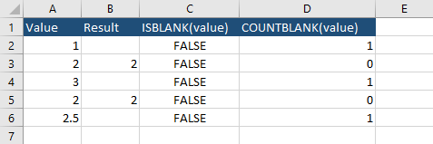
You can’t use the ISBLANK function because it will return FALSE for all cells. The better way here is to use the COUNTBLANK(value) formula. It checks whether the value of a cell is blank.
Let’s say, that you want to keep only the rows with blanks.
Select cells from D2 to D6 and use Ctrl + F. Enter “1” and click Find All. Select all the values and click Close.
In order to remove them, choose Ctrl + – and select Entire Row.
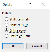
Now, you have only two rows left.

Make a cell truly blank cell
The above code works well, but there is another, more advanced way. This time the code leaves nothing inside a cell, not even a formula. It can’t be achieved only with formulas, we have to use a bit of the VBA code.
Let’s use the following example:
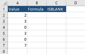
- Press Alt + F11 to open the VBA window.
- Create a new module and insert the following code.
|
1 2 3 4 |
Function DeleteCellContents(range) ThisWorkbook.Application.Volatile range.Value = "" End Function |
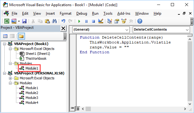
- Click cell A1 and go to Formulas -> Defined Names -> Name Manager. Click New.
Enter the following text in the fields.
Name: CreateTrueBlank,
Refers to:
|
1 |
=EVALUATE("DeleteCellContents("&CELL("address",Sheet1!A1)&")") |
- Enter the following code into B2:
|
1 |
=IF(A2=0,CreateTrueBlank,A2) |
Caution: This code won’t work if you start from A1 instead of A2 because we created a named range there.
Use Autofill, to fill the remaining cells.
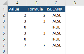
When you highlight cells B4 or B6 you can see that there is no formula there, and if you use the ISBLANK function you can see that this cell has nothing inside.
